
For better viewing, visit http://davidkun.github.io/HyperSpectralToolbox/
Originally created by Isaac Gerg and maintained by him here.
This repository is no longer being maintained or updated.
Isaac (the original creator of 99% of this work) has his own GitHub repository with this work and intends to actively maintain / update it there.
Please use that repository and see his BibTeX citation for correctly referencing the software in your research.
Dependencies
FastICA -- from Aalto University)
In the terminal type:
cd ~/path-to-directory
git clone https://github.com/davidkun/HyperSpectralToolbox.git
git clone https://github.com/davidkun/FastICA.git
Open Matlab. The default directory should contain a file startup.m. If not, create it:
% in Matlab command window
uPath = userpath;
cd(uPath(1:end-1)); % removes trailing colon
edit startup.m      % may ask if you'd like to create it; click Yes
Add the following code to it (make sure to modify path-to-directory so it matches the actual path):
addtopath('~/path-to-directory/FastICA', ...
          '~/path-to-directory/HyperSpectralToolbox/functions', ...
          '~/path-to-directory/HyperSpectralToolbox/newFunctions');
You're ready to go now! Check out the demo files hyperDemo.m in functions/ and hyperDemo2.m in newFunctions/ to learn how to use the toolbox, or see the examples further down this page.
The open source Matlab Hyperspectral Toolbox is a Matlab toolbox containing various hyperspectral exploitation algorithms. The toolbox is meant to be a concise repository of current state-of-the-art exploitation algorithms for learning and research purposes. The toolbox includes functions for:
- Target detection
- Constrained Energy Minimization (CEM)
- Orthogonal Subspace Projection (OSP)
- Generalized Likelihood Ratio Test (GLRT)
- Adaptive Cosine/Coherent Estimator (ACE)
- Adaptive Matched Subspace Detector (AMSD)
- Endmember Finders
- Automatic Target Generation Procedure (ATGP)
- Independent component analysis - endmember extraction algorithm (ICA-EEA)
- Material abundance map (MAM) generation
- Spectral Comparison
- Spectral angle mapper (SAM)
- Spectral information divergence (SID)
- Normalize cross correlation
- Anomaly Detectors
- Reed-Xiaoli Detector (RX)
- Least Square Solvers (for abundance map estimation)
- Fully-constrained least squares (FCLS)
- Non negative least squares (NNLS)
- Material Count Estimation
- HFC virtual dimensionality (VD) for material count estimate
- Automated processing
- Change detection
- Visualization
- Reading / writing files (.rfl, .asd, ect)
Download the Cuprite, Nevada hyperspectral image (HSI) from here. This will contain reflectance data and a .spc file with the spectral bands. The following samples of code are from hyperDemo2.m.
Show a 'slice' of the HSI:
slice = hyperReadAvirisRfl(rflFile, [1 512], [1 614], [bndnum bndnum]);
figure; imagesc(slice); axis image; colormap(gray);
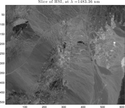
Figure 1: 1997 AVIRIS flight over Cuprite, NV
View an enhanced truecolor composite of the HSI:
tColor   = hyperTruecolor(rflFile, 512, 614, 224, rgbBands, 'stretchlim');
figure; imagesc(tColor); axis image
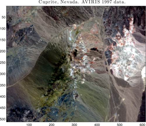
Figure 2: Truecolor composite from RGB bands
Plot the spectral signatures of 20 random pixels in order to determine which bands are greatly affected by water absorption and/or have a low signal-to-noise ratio (SNR):
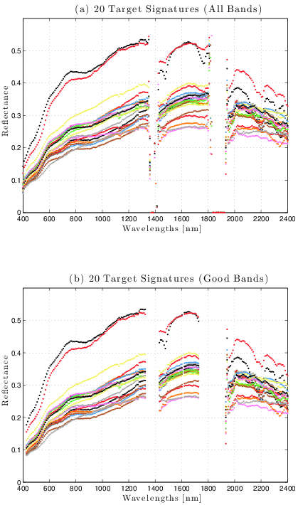
Figure 3: Pre-processing: removal of poor spectral bands from original HSI
Using the resampled HSI cube, perform an endmember extraction algorithm, for example, the N-FINDR algorithm:
Unfindr = hyperNfindr(M2d, q);
figure; plot(lambdasNm, Unfindr, '.'); grid on;
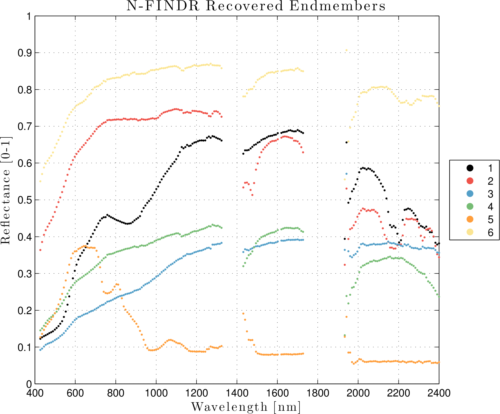
Figure 4: Endmember signatures estimated by PPI
Generate abundance maps using the non-negative constrained least squares method for each extracted endmember signature, for example:
abundanceMaps = hyperNnls(M2d, Uppi);
abundanceMaps = hyperConvert3d(abundanceMaps, h, w, q);
figure; imagesc(abundanceMaps(:,:,1)); colorbar; axis image;
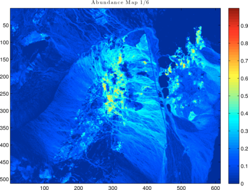
Figure 5: Abundance map from first N-FINDR-recovered endmember
These are just a few features of the Hyperspectral Toolbox.
(Joint) Affine Matched filter
Generalization of matched filter which includes signature statistics
RAF-SAM, an improvement to SAM from: Improving the Classification Precision of Spectral Angle Mapper
ELM for radiance to reflectance conversion - http://www.cis.rit.edu/files/197_SPIE_2005_Grimm.pdf
Covariance matrix inversion methods (e.g. Dominant Mode Rejection)
Quadratic Detector
SMACC - http://proceedings.spiedigitallibrary.org/proceeding.aspx?articleid=844250
AMEE - http://ieeexplore.ieee.org/xpl/articleDetails.jsp?arnumber=1046852
N-FINDR - http://proceedings.spiedigitallibrary.org/proceeding.aspx?articleid=994814
Fast PPI - http://ieeexplore.ieee.org/xpl/articleDetails.jsp?arnumber=1576691
Joshua Broaderwater's hybrid detectors (HUD, etc)
Variations on ACE - e.g. adaptive covariance estimated ACE, etc