spatialkit

Spatial tessellation, modeling, and cross-validation toolkit for R

The problem this solves

You have point observations — sites, sensors, parcels, plots — and you need to summarise or model them over areas. The path of least resistance is to borrow boundaries that already exist: ZIP codes, census tracts, counties, sales territories. Every one of those was drawn for mail routing, enumeration or politics, and none of them knows anything about the process you are studying. Aggregate to them and part of your answer is an artefact of the partition — the modifiable areal unit problem, and it is not a rounding error: the same observations can support materially different conclusions under different boundaries.

spatialkit lets the data draw the boundaries instead:

Seed cells where the observations actually are — get_voronoi_seeds() places seeds by k-means on the point cloud, so cell density follows sampling density rather than an inherited grid.
Let the geometry choose how many — determine_optimal_levels() ranks candidate cell counts by the elbow of within-cluster variance. Hand it a response as well and it additionally scores each partition by the spatial autocorrelation left in the residuals — informative only once there are more than about ten cells, for reasons spelled out under How many cells?. Better than picking a round number either way.
Build them, reproducibly — build_tessellation() produces Voronoi, hex, square or Delaunay cells, clipped to your study area, with stable IDs that do not shift when the input row order does.
Aggregate honestly — summarize_by_cell(deff = "kish") corrects cell-level standard errors for within-cell autocorrelation, rather than treating clustered observations as independent and reporting intervals that are too narrow.

Redrawing boundaries is easy; knowing whether the result means anything is not. So the second half of the package exists to keep you honest: three model backends — geographically weighted regression (GWmodel), a Bayesian spatial Gaussian process (brms), and random forests (ranger) — behind one spatial_fit S3 class so they can be scored on identical folds; cross-validation that holds out whole regions sized to the data's own autocorrelation range; and an area-of-applicability estimate that marks where the resulting score actually applies. All of it is built on sf, with CRS management that will not silently hand metres to a function expecting degrees.

That validation half matters more than it sounds. Fit something flexible, cross-validate it, get an R² of 0.8, predict onto a grid — and the map is wrong in ways the score never hinted at. The score was wrong because the folds were wrong. Random k-fold puts a test point's nearest neighbours in the training set, and under spatial autocorrelation those neighbours carry most of its signal. The model is scored on interpolation between known points while the actual task is extrapolation away from them. The same thing happens one level up, in variable selection: a predictor chosen by random inner folds can be chosen for leaking rather than for predicting.

Here is the gap, on 600 synthetic points with a smooth spatial field the predictor does not explain. Same data, same model, same settings — only the fold construction differs:

Fold scheme	Pooled out-of-sample R²	RMSE
`make_folds(method = "random_kfold")` (the default)	0.824	1.075
`make_folds(method = "block_kfold")`	0.379	2.129

library(spatialkit)
library(sf)

set.seed(42)
n     <- 600
x     <- runif(n, 0, 10000)
y     <- runif(n, 0, 10000)
field <- 3 * sin(x / 1500) * cos(y / 1500) + 2 * sin((x + y) / 4000)
site  <- st_as_sf(data.frame(elev = rnorm(n), x = x, y = y),
                  coords = c("x", "y"), crs = 32632)
site$price <- 10 + 1.5 * site$elev + field + rnorm(n, 0, 0.5)

random  <- make_folds(site, k = 5, method = "random_kfold", seed = 42)
blocked <- make_folds(site, k = 5, method = "block_kfold",  seed = 42)

# include_coords = TRUE lets the forest memorise location. That is the point:
# it is the failure mode the default (FALSE) exists to prevent, and the one
# random folds cannot see.
args <- list(include_coords = TRUE, num_trees = 300, seed = 1)
do.call(cv_rf, c(list(site, "price", "elev", folds = random),  args))$overall
do.call(cv_rf, c(list(site, "price", "elev", folds = blocked), args))$overall

More than half the reported skill was leakage. The gap is largest for models that can interpolate location directly — a forest handed the coordinates, a GWR, a Gaussian process — but it does not disappear when you leave the coordinates out. It just stops being visible unless you measure it.

make_folds()'s default is random_kfold, deliberately: it is the baseline you compare against, not the one to report.

Scope

Everything above is what the package is for. Here is where it stops, so you can rule it out now rather than after the quick start:

Regression only. A non-numeric response is refused outright, and an integer-coded binary response is refused by fit_gwr_model() with a pointer to GWmodel::ggwr.basic(). (A two-valued non-integer response — a measurement censored at a detection limit, say — is continuous, so it is fitted with a warning rather than refused.) There is no classification path.
Vector point data only. No raster support. predict_surface() returns an sf POINT layer, not a SpatRaster; convert downstream if you need one.
No areal / lattice models. Moran's I here is a residual diagnostic on point data. There is no CAR, SAR or spatial-lag fitter.
No spatio-temporal folds. Every fold scheme is purely spatial.

Installation

spatialkit is on CRAN:

install.packages("spatialkit")

That gets you 1.0.0 (published 2026-08-07). The development version below is ahead of it and changes several defaults — see NEWS.md before upgrading a running analysis.

# Development version from GitHub
# install.packages("remotes")
remotes::install_github("elkronos/gis_modeling_toolkit")

# With the vignette (needs pandoc)
remotes::install_github("elkronos/gis_modeling_toolkit", build_vignettes = TRUE)

# From a local clone
devtools::install("path/to/spatialkit")

Hard dependencies (sf, dplyr, logger, digest) install automatically. Everything else is in Suggests and checked at runtime:

Feature	Install
GWR modeling	`install.packages(c("GWmodel", "sp"))`
Bayesian GP modeling	`install.packages("brms")` (with `rstan`; or the non-CRAN `cmdstanr` backend if you have it)
Random forest modeling	`install.packages("ranger")`
Delaunay triangulation	`install.packages("geometry")`
Variogram autocorrelation range	`install.packages("gstat")`
PSIS-LOO information criterion	`install.packages("loo")`
Plotting	`install.packages("ggplot2")` (`patchwork` for multi-panel layouts)
k-NN weights for Moran's I above n = 5,000	`install.packages(c("FNN", "Matrix"))`
Tibble output from `make_folds()` / CV predictions	`install.packages("tibble")`

FNN and Matrix are not merely a speedup. residual_morans_i() errors above n = 5,000 without both: FNN supplies the kd-tree neighbour lookup and Matrix keeps the weight matrix sparse, and the fallback path allocates a dense n × n matrix. Below that threshold the fallback runs fine.

Quick start

This first block uses nothing outside the hard dependencies. It runs on a bare install.

library(spatialkit)
library(sf)

set.seed(1)
n  <- 400
df <- data.frame(x = runif(n, 0, 5000), y = runif(n, 0, 5000))
df$elev  <- rnorm(n)
df$price <- 50 + 0.004 * df$x + 3 * df$elev + rnorm(n)
pts <- st_as_sf(df, coords = c("x", "y"), crs = 32632)

# Voronoi cells grow from SEEDS, not from the observations themselves. Seeding
# one cell per point is a nearest-neighbour interpolation, not an aggregation:
# every cell holds one observation, so every ..sd_* / ..se_* column comes back
# NA and there is no within-cell variation to estimate an intra-class
# correlation from. `method = "kmeans"` will not hand you one seed per point
# whatever n you ask for; the way to reproduce that degenerate case
# deliberately is get_voronoi_seeds(method = "provided", seeds = pts).
seeds <- get_voronoi_seeds(sample_points = pts, method = "kmeans", n = 25)
tess  <- build_tessellation(seeds, method = "voronoi", quiet = TRUE)

assigned <- assign_features_to_polygons(pts, tess$cells, polygon_id_col = "cell_id")

# deff = "kish" widens the ..se_* columns by a design effect: the factor by
# which correlation between observations in the same cell shrinks the
# effective sample size, so an SE computed as if the n points were independent
# is too narrow. Standard errors are IID at the default deff = 1. The
# Diagnostics section below and ?summarize_by_cell cover how to read one.
cells <- summarize_by_cell(assigned, response_var = "price",
                           predictor_vars = "elev", deff = "kish")

head(as.data.frame(cells)[, c("cell_id", "n", "resp_mean_price",
                              "..sd_resp_price", "..se_resp_price")])
#>   cell_id  n resp_mean_price ..sd_resp_price ..se_resp_price
#> 1       1  7        51.44352        4.908403        4.204213
#> 2       2  4        51.60967        5.925025        5.188861
#> 3       3 11        53.47350        4.165362        3.528304

attr(cells, "deff_applied")$method
#> [1] "kish"

The second block fits and validates a model, on the site data built at the top of this file. It needs ranger, and gstat if you want the fold size derived from the data rather than chosen by hand. Swap fit_rf_model()/cv_rf() for fit_gwr_model()/cv_gwr() (GWmodel + sp) or fit_bayesian_spatial_model()/cv_bayes() (brms) — the surrounding code is identical.

# --- How big should a block be? Ask the data first --------------------------
# estimate_sac_range() fits a variogram to the OLS residuals and reports the
# distance at which spatial correlation dies out. It refuses to guess:
range <- estimate_sac_range(site, response_var = "price", predictor_vars = "elev")
range
#> NA
# It prints as a bare NA and nothing else. The diagnosis is in the attributes
# and in a logged WARN spelling out that the fitted range exceeds the largest
# lag the variogram covers (7043), so it is unidentified, not long:
attr(range, "rejected_range")    #> [1] 98348.32
attr(range, "rejected_reason")   #> [1] "fitted range exceeds the largest lag fitted"

# That NA is the correct answer, not a failure: this synthetic field is a smooth
# sinusoid that never levels off inside the study area, so its range is
# unidentified rather than long. `auto_range = TRUE` would ask the same question,
# log the same explanation, and fall back to geometric blocks -- so here we size
# the blocks ourselves and say so.
folds <- make_folds(site, k = 5, method = "block_kfold",
                    block_size = 2000, seed = 42)
folds$params$block_size   # what actually got used -- always worth checking
#> [1] 2000

# --- Fit, then cross-validate on those exact folds --------------------------
fit <- fit_rf_model(site, response_var = "price", predictor_vars = "elev")
cv  <- cv_rf(site, "price", "elev", folds = folds)
cv$overall        # pooled out-of-sample RMSE, MAE, R2, ...
cv$fold_metrics   # per-fold breakdown

# --- Residual spatial autocorrelation diagnostic ----------------------------
residual_morans_i(fit)
#> $observed [1] 0.7023314   $z [1] 36.3353   $p_value [1] 4.48e-289

A large positive residual Moran's I says the model has left spatial structure on the table — here, because elev is unrelated to the spatial field.

Compare backends on the same folds. Pass folds explicitly: without it each wrapper builds its own, and the comparison is between models and fold schemes:

comparison <- compare_models_cv(site, "price", "elev",
                                models = c("RF", "GWR", "Bayesian"),
                                folds = folds)
comparison$overall

models accepts any subset of c("GWR", "Bayesian", "RF") in any order. A backend whose package is not installed is dropped with a message, so the call still returns the models that could run — but only if at least one survives. Drop them all and the call errors:

compare_models_cv(site, "price", "elev", models = c("GWR", "Bayesian"), folds = folds)
#> compare_models_cv(): dropping GWR (package/function unavailable).
#> compare_models_cv(): dropping Bayesian (package/function unavailable).
#> Error: compare_models_cv(): no viable models.

Backend-specific arguments go in gwr_args, bayes_args and rf_args. Which backend to reach for, and what each one costs, is Choosing a backend.

Your own data

Everything above manufactures its data inline so it runs on a bare install. Your data arrives through one of two doors, and both end in the same place: an sf object of POINTs in a projected CRS.

library(spatialkit)
library(sf)

# --- Door 1: a spatial file (shapefile, GeoPackage, GeoJSON, ...) -----------
nc <- st_read(system.file("shape/nc.shp", package = "sf"), quiet = TRUE)

# nc.shp holds polygons; every model here takes point observations, so reduce
# them first. coerce_to_points() maps a polygon to a point guaranteed to lie
# inside it (st_point_on_surface()), a line to its midpoint and a MULTIPOINT
# to its centroid, keeping the attribute columns.
# ensure_projected() logs which CRS it chose and why -- see the next section.
counties <- ensure_projected(nc[, c("BIR74", "SID74")])
obs      <- coerce_to_points(counties)

# Hex and square grids need a study area. Dissolving the source polygons is
# the usual way to get one; st_read() a separate outline if you have it.
boundary <- st_as_sf(st_union(counties))

# --- Door 2: a table with coordinate columns -------------------------------
# (a stand-in for your own file; `tab` is what read.csv() would hand you)
csv <- tempfile(fileext = ".csv")
write.csv(data.frame(lon    = st_coordinates(st_transform(obs, 4326))[, 1],
                     lat    = st_coordinates(st_transform(obs, 4326))[, 2],
                     births = obs$BIR74,
                     sids   = obs$SID74),
          csv, row.names = FALSE)

tab <- read.csv(csv)
head(tab, 2)
#>         lon      lat births sids
#> 1 -81.49692 36.41746   1091    1
#> 2 -81.12964 36.47430    487    0

# `crs =` is not optional and cannot be guessed. Lon/lat from a GPS, a web
# API or a geocoder is almost always EPSG:4326; if the file came from a
# municipal or national dataset, the metadata names the CRS and it is
# frequently not 4326.
nc_pts_ll <- st_as_sf(tab, coords = c("lon", "lat"), crs = 4326)
nc_pts    <- ensure_projected(nc_pts_ll)

ensure_projected() is the only step people skip, and it is the one that decides what every distance in the package means.

CRS: what the numbers are in

Block sizes, buffers, expand distances, GWR bandwidths and variogram ranges are all plain numbers in the units of the working CRS. Nothing in the package is in metres by default, and projected does not mean metric — EPSG:2264, used by the vignette and the demo script, is in US survey feet. st_crs(x)$units_gdal tells you which.

Geographic (lon/lat) input is projected automatically, because degrees are not a length: estimate_sac_range(), the distance-based make_folds() methods, every fit_*() (via prep_model_data()) and predict_surface() route their input through ensure_projected() before measuring anything. The CRS it picks is chosen for your extent — a UTM zone from the data's centroid when the extent is narrow enough for one, an equal-area projection centred on the data when it is not, because forcing continental-width data into a single UTM zone costs percent-scale distance errors that propagate silently into ranges, block sizes and bandwidths. It says which, and why:

nc_pts <- ensure_projected(nc_pts_ll)
#> WARN  .pick_local_projected_crs(): extent reaches 5.1 deg from the central
#> meridian of UTM zone 17, well beyond the 3 deg the zone is designed for
#> (8.1 deg longitude span in total). Using Albers equal-area (lat_1=34.5,
#> lat_2=36.1, lon_0=-79.5) instead; ... Pass target_crs to ensure_projected()
#> to override.

st_crs(nc_pts)$units_gdal
#> [1] "metre"

Two consequences worth internalising:

Project before you choose a number. make_folds(nc_pts_ll, block_size = 2000) succeeds on lon/lat input, and the 2000 is in metres of a CRS you never chose. Call ensure_projected() yourself, look at st_bbox(), and pick block_size against that. folds$params$crs records the CRS the folds were actually built in, which is the one block_size was in.
Pin the CRS when it matters. ensure_projected(x, target_crs = 2264) or build_tessellation(..., crs = 2264) forces a specific one, which is what you want when results have to line up with an existing analysis, a published bandwidth, or a colleague's grid.

Which function do I want?

I want to…	Use
get my data into a projected CRS	`ensure_projected()`, `coerce_to_points()`, `harmonize_crs()`
cut my study area into cells	`build_tessellation()` (`"voronoi"`, `"hex"`, `"square"`, `"triangles"`)
place the seeds a Voronoi grows from	`get_voronoi_seeds()`
choose how many cells	`determine_optimal_levels()`
put points into cells and aggregate	`assign_features_to_polygons()` → `summarize_by_cell()`
draw the result	`plot_tessellation_map()`
know how far spatial correlation reaches	`estimate_sac_range()`
build honest CV folds	`make_folds()` (`random_kfold`, `block_kfold`, `buffered_loo`, `leave_location_out`, `nndm`)
see whether my folds actually separate	`plot_folds()`
fit a model	`fit_gwr_model()`, `fit_bayesian_spatial_model()`, `fit_rf_model()`
score it out of sample	`cv_gwr()`, `cv_bayes()`, `cv_rf()`
score my own learner on the same folds	`cv_spatial()` + `new_spatial_fit()`
score it in sample	`model_metrics()`, `evaluate_insample()`, `compare_models()`
pick predictors without leaking	`select_features_forward()` (`gwr_model_selection()` for the AICc counterpart)
compare backends head to head	`compare_models_cv()`
check for leftover spatial structure	`residual_morans_i()`, `plot(fit, type = "variogram")`
turn a fit into a map	`predict_surface()`
know where that map is extrapolation	`area_of_applicability()`
free memory held by the caches	`clear_grid_cache()`, `clear_fitted_cache()`

The lower-level exports behind these — create_voronoi_polygons(), create_grid_polygons(), create_grid_polygons_cached(), clip_target_for(), ensure_stable_poly_id(), voronoi_seeds_kmeans(), voronoi_seeds_random(), prep_model_data() and gp_lengthscale_bounds() — are exported and documented too; help(package = "spatialkit") lists everything.

The `spatial_fit` interface

All three backends return an object inheriting from spatial_fit, so predict(), fitted(), residuals(), summary() and model_metrics() work the same way on all of them. Two caveats are real and worth stating up front:

coef() is not universal. coef.rf_fit() errors by design — a forest has no coefficients. Use fit$info$importance (permutation importance) instead. coef.gwr_fit() returns the local coefficient frame and coef.bayesian_fit() the fixed-effect posterior summary; both stop() when the backend cannot supply them rather than returning NULL, so lapply(fits, coef) never silently returns a short answer. Wrap in try() when sweeping a heterogeneous list.
summary() does not mean the same thing on every backend. fitted.rf_fit() returns out-of-bag predictions, not in-sample ones, so summary() on an rf_fit reports out-of-bag metrics (and says so). A gwr_fit and a bayesian_fit report genuinely in-sample metrics. The two are not comparable. Use compare_models_cv(), which scores every backend the same way. The flag is fit$info$fitted_are_oob.

Extending it: your own learner on the same folds

cv_spatial() is the extensibility point. Pass any fit_fn(train_sf) that returns a spatial_fit, built with the new_spatial_fit() constructor, and it plugs into the same folds, metrics and comparison tooling:

lm_fit <- function(train_sf) {
  new_spatial_fit(
    subclass       = "lm_fit",
    engine         = lm(price ~ elev, sf::st_drop_geometry(train_sf)),
    formula        = price ~ elev,
    response_var   = "price",
    predictor_vars = "elev",
    data_sf        = train_sf
  )
}
predict.lm_fit <- function(object, newdata = NULL, ...)
  as.numeric(stats::predict(object$engine, sf::st_drop_geometry(newdata)))

cv <- cv_spatial(site, "price", "elev", fit_fn = lm_fit, folds = blocked)
cv$overall
cv$n_folds_attempted  # compare against n_folds_succeeded before trusting the above

fit_fn is called on the training slice only, so anything you do inside it — scaling, tuning, an inner feature sweep — is already nested and leak-free.

Tessellation

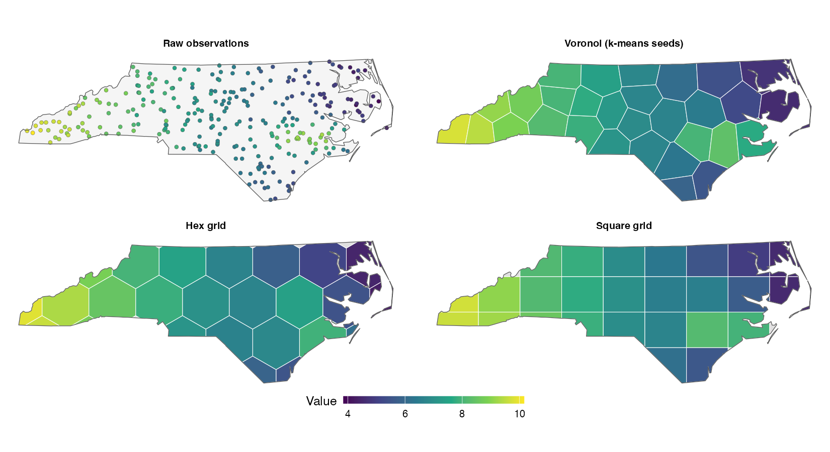
build_tessellation() offers four methods. Below, three of them cut the same geography. The first panel shows raw observations of a smooth spatial field over North Carolina (high in the west, with an eastern hotspot). The others show the same points aggregated into Voronoi regions grown from k-means seeds, a hex grid, and a square grid — each cell coloured by the mean of the points inside it (assign_features_to_polygons() + summarize_by_cell()). All panels share one colour scale, so each tessellation should look like a mosaic version of the raw data:

All four methods return cells carrying a cell_id column, so downstream code and plot_tessellation_map(fill_col = "cell_id") treat them alike; hex and square grids additionally keep poly_id, holding the same values.

Which method?

Method	A cell is	Reach for it when
`"voronoi"`	the area closer to one seed than to any other seed	cells should follow sampling density — small where you sampled densely, large where you did not. Seeds come from `get_voronoi_seeds()`; the observations themselves are not the seeds.
`"hex"`	one hexagon of a regular lattice over the boundary	you need a regular lattice: comparable cell areas and equal-distance neighbours, so cell size cannot confound the map
`"square"`	one square of a regular lattice over the boundary	the same, and the cells have to line up with an existing raster or grid
`"triangles"`	one Delaunay triangle of the input points	you want the point-triplet structure itself — adjacency, interpolation supports — rather than an aggregation

The practical split is whether the sampling design carries information you want the partition to inherit. If it does, Voronoi. If it does not — and unequal cell areas would be an artefact rather than a feature — hex or square.

"triangles" is the odd one out: a Delaunay triangulation of n points has roughly 2n triangles (300 points gave 586 in the demo script), so its cells are far finer than the other three and most hold barely any data. summarize_by_cell() needs several points per cell to say anything, which rules "triangles" out for aggregation.

Hex and square grids need a boundary

Voronoi and Delaunay take their extent from the points themselves — Voronoi falls back to their convex hull when you pass no boundary. A grid cannot: nothing in a point cloud says where a lattice should stop. Both grid methods therefore require boundary, and say so rather than guessing:

build_tessellation(obs, method = "hex", approx_n_cells = 40)
#> Error: build_tessellation(): `boundary` is required for hex/square grids.

hex <- build_tessellation(obs, boundary = boundary, method = "hex",
                          approx_n_cells = 40, clip = TRUE, quiet = TRUE)
nrow(hex$cells)
#> [1] 38

(obs and boundary are from Your own data above.) approx_n_cells is a target, not a promise: clip = TRUE intersects the lattice with the boundary and drops what falls outside, so the count comes back near, not at, what you asked — the same call with method = "square" returns 32. Pass cellsize instead when the cell edge, in CRS units, is the thing you need to hold fixed.

How many cells?

Resolution is a modeling decision, not a cosmetic one: too few cells smooth the signal away, too many leave each cell with a handful of noisy observations. determine_optimal_levels() offers two criteria and their combination. The geometric one — criterion = "geometric" — takes the elbow of the within-cluster sum of squares from a k-means sweep. The model-aware one — criterion = "morans_i" — aggregates to cell means at each candidate k, fits OLS, and computes Moran's I on the residuals, so it prefers the resolution that leaves the least unexplained spatial structure. "combined" rank-averages the two. "geometric" is the default, but supplying response_var and predictor_vars auto-upgrades it to "combined" with a logged note — so the model-aware half is on whenever you hand it a model, whether you asked or not.

It returns a vector of top_n candidates (default 3), best first — not a single number:

k <- determine_optimal_levels(pts, response_var = "price",
                              predictor_vars = "elev", max_levels = 15,
                              criterion = "combined")
#> WARN  determine_optimal_levels(): Moran's I could not be computed;
#> falling back to geometric.
k
#> [1] 3 4 5
k[1]                          # the top-ranked candidate
#> [1] 3

Below ten cells, the elbow does all of the work — and that is most calls. Moran's I here runs over a k-nearest-neighbour graph on the cell centroids with min(8, n_cells - 1) neighbours, so at nine cells or fewer every cell neighbours every other one. On a complete, row-standardised graph Moran's I collapses to exactly -1/(n_cells - 1) for any residual vector — the null expectation, carrying nothing about your data — and |I| then falls monotonically in k for purely arithmetic reasons, which would rank the largest candidate first every time. Rather than report that, the model-aware criteria return NA below the floor; when no candidate clears it, the whole call falls back to the geometric ranking and logs the warning above. That is what happened here: max_levels = 15, but the search only evaluates a window around the elbow, and that window sat entirely inside the degenerate zone.

So: use the elbow to pick resolution, and treat the residual-autocorrelation criterion as something that only starts contributing above roughly ten cells. Raise max_levels until the elbow neighbourhood reaches past it and the diagnostics fill in:

k <- determine_optimal_levels(pts, response_var = "price",
                              predictor_vars = "elev", max_levels = 40,
                              criterion = "combined")
as.integer(k)     # printing `k` itself dumps the diagnostics attribute too
#> [1]  5  6 10

d <- attr(k, "diagnostics")             # present only when Moran's I ran
round(d$moran_i[d$eval_ks], 4)
#> [1]     NA     NA     NA     NA     NA     NA     NA 0.0135 0.0411

Seven NAs for k = 3..9, then two real values at k = 10 and 11. Only those two carry information, and both are near zero — this synthetic field leaves little residual structure at either resolution, so the elbow keeps the final say.

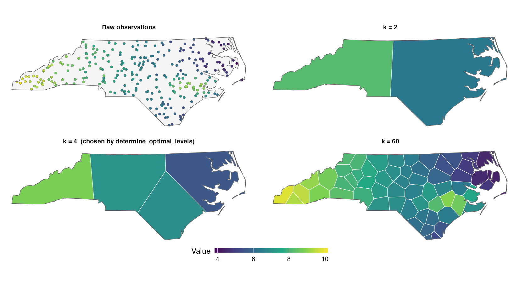
The same field cut at three resolutions, next to the raw observations — too coarse blurs the hotspot, too fine chases noise with near-empty cells, and the selected k preserves the trend without overfitting geography:

Cross-validation

make_folds() offers five schemes:

Method	Holds out	Use when
`random_kfold` (default)	a random 1/k of rows	you want the optimistic baseline to compare against
`block_kfold`	contiguous spatial blocks	the general case; size blocks from `estimate_sac_range()` via `auto_range = TRUE`
`buffered_loo`	one point, plus everything within `buffer`	leave-one-out with an explicit exclusion radius
`leave_location_out`	every observation from one site (`group_var`)	repeated measurements at the same locations
`nndm`	one point, plus a distance-matched exclusion	you know where you will predict; pass `prediction_points`

nndm implements Milà et al. (2022): rather than picking a buffer with nothing to justify it, the exclusion around each held-out point is sized so the training-to-test distance distribution reproduces the distances from your actual prediction locations to the training data. params$target_median and params$realised_median record how close the match came.

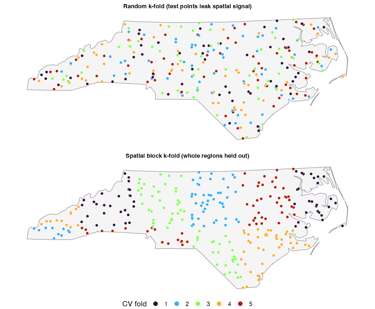
The difference is easy to see. On the same North Carolina sites, random folds scatter test points among their spatially correlated training neighbours, while block folds hold out contiguous regions:

make_folds() may return fewer folds than requested — block_kfold when the grid yields fewer non-empty blocks, leave_location_out when there are fewer distinct groups, and buffered_loo/nndm always return k = n. Read folds$k rather than assuming.

Choosing `k` and `block_size`

For block_kfold these two arguments pull against each other, and the tension is the whole design problem:

block_size too small and a held-out block is narrower than the autocorrelation range, so training points just outside it still carry the test points' signal. Leakage creeps back and you have paid for blocking without buying anything. The block has to be wider than the range for the hold-out to mean "somewhere the model has not been".
k too small and each fold trains on (k-1)/k of the data — at k = 3, two-thirds — so the score is of a model fitted on much less data than the one you will ship, and pessimistic for that reason rather than for a spatial one. Few folds also means few blocks, and a fold-to-fold spread computed from three numbers.
k too large and, at a fixed study area, the blocks shrink back below the range. k = 10 on a small extent is often just random_kfold with extra steps.

estimate_sac_range() is the anchor: get the range, make block_size comfortably larger than it, then let k be whatever the extent supports at that size. k = 5 is a reasonable default to start from. auto_range = TRUE does the first two steps for you — and, crucially, tells you when it could not:

folds <- make_folds(site, k = 5, method = "block_kfold",
                    auto_range = TRUE, response_var = "price",
                    predictor_vars = "elev", seed = 42)
#> WARN  make_folds(block_kfold): auto_range requested but estimation
#> returned NA; falling back to geometric blocks.

folds$k                    # may be lower than requested
#> [1] 5
folds$params$block_size    # NULL here -- the range was never identified
#> NULL

So always read both back. plot_folds() is the fastest check that the blocks separate anything at all.

When `estimate_sac_range()` returns `NA`

An NA is a refusal, not a failure: the empirical variogram never levelled off, so the fitted range sits beyond the largest lag it was fitted over and is unidentified rather than long. Handing that number to make_folds() would size blocks from an artefact. The logged warning names three next steps, in the order worth trying:

Raise cutoff. It is a fraction of the maximum inter-point distance, default 0.5, so lags beyond half the study extent are never fitted. If the sill is genuinely further out, cutoff = 0.8 lets the fit see it — at the cost of the noisiest, sparsest lags, which is why it is not the default.
Supply predictor_vars. The variogram is fitted to OLS residuals. A large-scale trend the predictors would absorb otherwise looks like autocorrelation that never decays — detrending is frequently the whole fix.
Set block_size explicitly and say in your write-up that you did. A defensible starting point is a fraction of the study extent — one fifth of the shorter bbox side gives roughly 5 x 5 blocks — sanity-checked with plot_folds().

What you should not do is treat NA as "no autocorrelation" and fall back to random_kfold. An unidentified range usually means correlation reaching past the study area, which is the case where random folds are most optimistic.

Choosing a backend

compare_models_cv() scores all three on identical folds and is the right answer when you can afford it. It is not always cheap. On the recorded baselines (dev/baseline-accuracy.rds: one machine, one run, 4-fold CV, 2 chains × 1,000 iterations) the Bayesian GP took 1,186 s at n = 2,000 against 109 s for cv_gwr() on the same data — and at n = 300, 142 s against 0.8 s, so the ratio is not fixed either. A cv_rf() of the same shape is seconds. So it is worth knowing what each backend is for before you spend an afternoon comparing them:

Backend	Reach for it when you want	Cost
GWR (`fit_gwr_model()`, `GWmodel` + `sp`)	spatially varying coefficients you can interpret and map — "the elevation effect is strong in the west and absent in the east" is the answer only this one gives	moderate; grows quickly with n
Bayesian spatial GP (`fit_bayesian_spatial_model()`, `brms`)	calibrated uncertainty: posterior predictive intervals, `se = TRUE` surfaces, CRPS. Also the natural spatial null — `predictor_vars = character(0)` fits an intercept-only GP, which asks how much of the surface is spatial structure rather than covariate effect	far the highest; every CV fold is a full MCMC run
Random forest (`fit_rf_model()`, `ranger`)	nonlinearity and interactions without specifying them, and no inference — permutation importance is what you get instead of coefficients	far the lowest; the one to prototype with

Two things that are not backend choices. First, none of them fixes bad folds — all three can interpolate location directly, which is where the gap at the top of this file is widest, so the fold scheme has to be right before the backend comparison means anything. Second, if the question is only "is there spatial structure my predictors miss", residual_morans_i() on the cheapest fit you can make answers it before you pick anything.

Prediction

All three backends support true out-of-sample prediction — newdata needs only the predictor columns and geometry, not the response:

new_sites <- st_sf(
  elev = c(0.5, -1.2),
  geometry = st_sfc(st_point(c(1000, 2000)), st_point(c(3000, 4000)), crs = 32632)
)
predict(fit, newdata = new_sites)

newdata is automatically transformed to the CRS used during fitting, rows with missing or non-finite predictors return NA (output length always matches nrow(newdata)), and non-point geometries are coerced to representative points. A length mismatch between the predictions and the rows that survived cleaning is an error, never a silent recycle. The Bayesian method additionally supports type = "predict" for full posterior predictive draws and draws = TRUE for the raw draw matrix; both are honoured with newdata = NULL as well.

model_metrics() does require the response in newdata, since it computes error metrics against observed values.

Prediction surfaces

Building newdata by hand is the fiddly part of producing the thing most people actually want from a fitted spatial model — a map. predict_surface() builds a regular grid over the training extent, joins covariates from the nearest feature, clips to a boundary, predicts in chunks and returns sf:

surf <- predict_surface(fit, n_cells = 2000, covariates = site)
plot(surf[".pred"])

Chunking matters for bayesian_fit, where the posterior draw matrix is n_draws x n_newdata and a fine grid would exhaust memory long before the fit itself would. Pass se = TRUE for a posterior-SD surface where the backend exposes draws, and boundary = a polygon to clip to a study area.

Diagnostics & statistical notes

Residual spatial autocorrelation

residual_morans_i() computes Moran's I on model residuals with the Cliff & Ord randomisation variance, using row-standardised k-NN weights by default (sparse via FNN + Matrix when available) or a user-supplied weight matrix (base or sparse Matrix). compare_models() runs it automatically and logs a warning when residual spatial structure remains.

Aggregation standard errors

Aggregation standard errors are IID unless you ask otherwise. The ..se_* columns from summarize_by_cell() are IID standard errors at the default deff = 1, which is anticonservative under within-cell spatial correlation. Autocorrelation-aware standard errors are opt-in: pass deff = "kish" to apply Kish's design-effect correction from estimated intra-class correlations (separate ICCs for response and predictors), a fixed numeric design effect, or deff = "variogram" to compute it from a fitted variogram instead of one pooled correlation. Kish assumes every pair in a cell is equally correlated regardless of separation, an assumption that degrades as cells grow; the variogram option lets correlation decay with distance, which is what having fitted a variogram is for. Substituting a constant off-diagonal correlation recovers Kish exactly. Inspect what was applied via attr(result, "deff_applied").

Reading a design effect. A design effect is a variance multiplier, so standard errors move by its square root. Kish's is deff_i = 1 + (n_i - 1) * rho per cell, from the intra-class correlation rho.

deff ≈ 1 — no within-cell correlation worth correcting for. The IID standard errors were already right.
deff = 4 — the cell's n points carry the information of n/4 independent ones, and its standard error is 2x the IID figure.

The demo script (inst/scripts/example_nc_demo.R, 300 points in 40 Voronoi cells) prints ICC(response) = 0.742 | median deff = 5.45 and a median response-SE inflation of 2.33x, which is sqrt(5.45). That is a strongly clustered response: at ~7.5 points per cell, each cell carries the information of fewer than two independent observations.

Cell size is the lever, and it moves the wrong way from most people's intuition. deff rises with cell occupancy, so bigger cells are worse. Re-running the demo's aggregation at other seed counts, same data, same seed:

Voronoi cells	mean points/cell	ICC	median `deff`	SE inflation
10	30.0	0.665	21.28	4.61x
20	15.0	0.714	9.93	3.15x
40	7.5	0.742	5.45	2.33x
80	3.8	0.780	3.34	1.83x
120	2.5	0.790	1.79	1.61x

So there are two honest responses, and picking between them is a modeling decision, not a formatting one:

Accept the wider intervals. They are the correct ones. If the conclusion survives them, it was never resting on the correlation. A large deff is not a bug and not a warning — it is the price of cells big enough to hold correlated observations, and it was always being paid; deff = 1 just did not show it on the invoice.
Use more, smaller cells (raise n in get_voronoi_seeds(), or a finer grid) so that less spatial variation is trapped inside a cell, where it only inflates deff, and more of it lands between cells, where it is estimated. That costs precision on each individual cell mean, so it is a trade, not a free win — and it does not manufacture information the correlated sample never had. Nothing but more spatially independent sampling does that.

If cells are large enough that "every pair inside is equally correlated" stops being credible, switch to deff = "variogram", which lets the correlation decay with distance instead.

Area of applicability

A fitted model returns a number for any location you hand it, including locations whose predictor values look nothing like anything it was trained on. Those predictions are extrapolations dressed as interpolations, and a cross-validation score says nothing about them — the held-out folds were drawn from the same predictor distribution as the training data. area_of_applicability() implements the dissimilarity index of Meyer & Pebesma (2021) and marks where the score applies:

surf <- predict_surface(fit, n_cells = 2000, covariates = site)
aoa  <- area_of_applicability(surf, model = fit, folds = folds)

# AOA is NA wherever a predictor was NA or non-finite. `!NA` is NA, and R
# silently skips NA positions in a subscripted assignment, so test for TRUE
# explicitly and let anything else count as outside.
inside <- aoa$aoa$AOA %in% TRUE
surf$.pred[!inside] <- NA          # blank out the extrapolations

Pass the make_folds() result you actually validated with. Without it the reference distance is each training point's nearest neighbour anywhere in the data, which for clustered data is very close, giving a conservative area; with it the reference distances are larger and the area is correspondingly wider. That is not a loophole — the area of applicability is defined relative to a performance estimate, and a spatially blocked estimate is a claim about predicting further away.

Leakage: coordinates and variable selection

Random forests and location. fit_rf_model() defaults to include_coords = FALSE. Handing a forest the x and y coordinates lets it reproduce the training surface almost exactly by memorising location, then fail badly anywhere it has not seen; random cross-validation does not catch this, because nearby points leak between folds (Meyer et al. 2019). That is the effect measured in the table at the top of this file. And summary()'s out-of-bag error is no substitute: OOB is itself a random hold-out, so it is optimistic under spatial autocorrelation for exactly the reason random k-fold is. Use cv_rf() for a blocked estimate.

Variable selection. select_features_forward() scores candidates against spatially blocked inner folds, which is the entire point of having it: random inner folds inside blocked outer folds select variables that look predictive only because nearby points leak between train and test, and the outer loop then reports honest-looking numbers for a dishonestly chosen feature set. Every candidate set is scored on the same rows, so a variable cannot win by having an easier surviving subset. gwr_model_selection() is the fast in-sample counterpart — the same forward search scored by AICc — and is worth cross-checking against the blocked estimate when the answer matters.

Backend-specific notes

GWR collinearity. fit_gwr_model() checks the global condition number of the predictor matrix and spot-checks local condition numbers within bandwidth windows at sampled locations, since spatially clustered subsets can be collinear even when the global matrix is not.

GWR bandwidth fallback. If automatic bandwidth selection fails, a heuristic fallback is used, a warning() is raised, and fit$info$bandwidth_is_fallback = TRUE is set so downstream comparisons can flag the result. Supply an explicit bandwidth if you see this.

Bayesian GP anisotropy. fit_bayesian_spatial_model() standardizes X and Y coordinates independently before the GP term, as a conditioning step — easting and northing often span very different ranges in a projected CRS. Because the axes are scaled separately, a single shared length-scale would make the kernel anisotropic in the original CRS by the arbitrary ratio sd(X)/sd(Y), which reflects the sampling layout rather than the process. The GP therefore fits one length-scale per axis by default (gp_iso = FALSE), estimating directional structure from the data; pass gp_iso = TRUE for a single shared length-scale. The scaling strategy is recorded in fit$info$coord_scaling$scaling_type, and a data-informed length-scale prior is derived from the inter-point distance distribution (see gp_lengthscale_bounds()). The spatial null noted under Choosing a backend is spelled predictor_vars = character(0).

Troubleshooting

The handful you are most likely to meet, and what each is actually telling you.

build_tessellation(): boundary is required for hex/square grids. A lattice has no extent of its own. Pass boundary = a polygon — dissolving your source polygons with st_union() is the usual way to get one. Voronoi and "triangles" do not need it; Voronoi falls back to the convex hull of the points.

prep_model_data(): missing required column(s): X A response_var or predictor_vars name that is not in the data. Usually a typo, a case difference, or a column renamed by read.csv()'s check.names = TRUE (pop density becomes pop.density). Check names(data_sf). The geometry column is not a predictor.

fit_rf_model(): response 'y' is not numeric. (And its fit_gwr_model() / fit_bayesian_spatial_model() equivalents.) Everything here is regression. A factor or character response is refused outright; a response that came back as character from a CSV needs as.numeric() first — check for a stray thousands separator or "NA" string if that produces NAs. fit_gwr_model() additionally refuses an integer-coded two-valued response and points at GWmodel::ggwr.basic().

n = 6000 requires FNN for k-NN weights, and Matrix to hold them sparsely residual_morans_i() above n = 5,000. The fallback allocates a dense n x n matrix, which is why this is an error rather than a slow path. install.packages(c("FNN", "Matrix")) — both, not either.

compare_models_cv(): no viable models. Every requested backend was dropped: unrecognised names raise a warning, uninstalled backends print dropping <name> (package/function unavailable). Read the messages immediately above the error — they name each one. Install the backend, or request one you have.

cv_*(): all folds failed; cross-validation results contain no predictions. A warning, not an error: $overall comes back all-NA with n_pred = 0. The per-fold WARN lines name the cause — a missing backend most often, but also a degenerate training slice or a predictor constant within a fold. Compare cv$n_folds_succeeded against cv$n_folds_attempted on every run, not just when something looks wrong: a partial failure produces a plausible-looking score computed from fewer folds than you asked for.

estimate_sac_range() returned NA. Not a failure — a refusal to report an unidentified range. See When estimate_sac_range() returns NA.

determine_optimal_levels(): Moran's I could not be computed; falling back to geometric. Every candidate resolution sat below the nine-cell floor where Moran's I is arithmetically degenerate. Expected at small max_levels; see How many cells?.

Distances, bandwidths or block sizes look absurd. Check the working CRS first: st_crs(x)$units_gdal. A block size that made sense in metres is meaningless in US survey feet, and lon/lat input gets projected to a CRS the package chose. See CRS: what the numbers are in.

Running it in practice

Three concerns that show up once the pipeline works rather than while you are building it: making cross-validation finish sooner, not recomputing what has not changed, and seeing what the package is doing.

Parallel cross-validation

Every CV function — cv_gwr(), cv_bayes(), cv_rf() and cv_spatial() — accepts a parallel argument for fold-level parallelism via parallel::mclapply() (macOS/Linux; falls back to sequential on Windows with a message). This matters most for cv_bayes(), where every fold is a full MCMC run:

# cv_bayes() needs `brms`. Without it every fold fails and you get an empty
# result, not an error -- a per-fold WARN naming the cause, one summarising
# R warning(), and $overall all-NA with n_pred = 0:
cv <- cv_bayes(site, "price", "elev", k = 5, parallel = TRUE)  # auto-detect cores
#> WARN  .cv_run_folds(): fold 1 fit failed; skipping.
#>       Cause: fit_bayesian_spatial_model(): package 'brms' is required.
#> ... (once per fold)
#> Warning: cv_bayes(): all folds failed; cross-validation results contain no
#> predictions. First error: fit_bayesian_spatial_model(): package 'brms' is required.

cv <- cv_rf(site, "price", "elev", k = 5, parallel = 4L)       # explicit count

Check cv$n_folds_succeeded against cv$n_folds_attempted before you read cv$overall. Every CV function records both, precisely because a partial or total fold failure degrades rather than errors — a missing backend is only the loudest cause; a fold whose training slice is degenerate fails the same way and leaves the remaining folds looking fine.

Results are reproducible from seed and identical to parallel = FALSE: one RNG stream per fold is drawn in the parent process, so each fold's stream is a function of (seed, fold index) alone.

Caching

Grid construction and posterior expectations are both expensive enough to memoise, so both are cached:

create_grid_polygons_cached() memoises grids keyed on boundary geometry, CRS, target cell count and arguments. clear_grid_cache() empties it.
fitted() on a bayesian_fit memoises posterior_epred() column means in an environment carried on the object, because summary(), residuals(), model_metrics() and compare_models() each call fitted() independently. clear_fitted_cache(fit) drops it — needed only if you mutate the engine or the training data by hand after fitting.

Logging

Detailed diagnostics are logged to a session temp file, and warnings are echoed to the console. Logging is scoped to the "spatialkit" namespace and never touches your global logger configuration. To customize:

logger::log_appender(logger::appender_file("my_analysis.log"), namespace = "spatialkit")
logger::log_threshold(logger::WARN, namespace = "spatialkit")

Note that these are logger messages, not R conditions: tryCatch(warning = ) will not catch them and suppressWarnings() will not suppress them. Where the documentation says a function raises a warning, it means a genuine R warning(); where it says a function logs one, it means this.

Development

devtools::load_all()   # interactive development
devtools::test()       # run the test suite
devtools::document()   # regenerate NAMESPACE + man/ from roxygen2 (7.3.1)
devtools::check()      # full R CMD check (vignette build requires pandoc)

The checked-in NAMESPACE and man/ are generated by roxygen2 7.3.1 (RoxygenNote in DESCRIPTION); devtools::document() reproduces them.

The README figures are generated from actual package output; regenerate them with Rscript dev/make_readme_figures.R. readme-resolution.png labels the cell count determine_optimal_levels() chose for that data, so it goes stale whenever that function's answer changes and must be rebuilt alongside it.

The test suite covers the geometry/tessellation pipeline, every exported function, and targeted regression tests for the statistical internals (Moran's I variance and its sparse-weights path, CV fold/row-ID alignment, CRPS, hex-grid sizing, CRS selection at wide extents, prediction CRS and NA alignment, and more). Tests that need an optional backend skip automatically when it is absent, and the backends job in R-CMD-check.yaml installs every optional backend except brms, so a green matrix means those guarded paths actually ran. brms is the thin spot: its Stan smoke tests are additionally gated behind the SPATIALKIT_TEST_BRMS environment variable, which only the weekly check-brms workflow sets, so they do not run in the matrix even where brms is installed.

Contributions are welcome — please open an issue describing the bug or proposed change, and include a regression test with any fix.

Project

Documentation

?spatialkit is the package-level page: it walks the pipeline in order and names the function that performs each step.
Every exported function is documented: see ?fit_gwr_model, ?make_folds, ?area_of_applicability, etc.
A worked end-to-end demo on the North Carolina boundary shipped with sf runs as a vignette: vignette("spatialkit_nc_demo") after installing with build_vignettes = TRUE.
A runnable script version is installed with the package: system.file("scripts", "example_nc_demo.R", package = "spatialkit").

Citation

citation("spatialkit")

The package entry cites spatialkit itself. citation() also prints the method references you should cite alongside it if you rely on area_of_applicability() (Meyer & Pebesma 2021), make_folds(method = "nndm") (Milà et al. 2022), the Bayesian GP basis (Riutort-Mayol et al. 2023), permutation importance in fit_rf_model() (Strobl et al. 2007), coordinate predictors and blocked validation (Meyer et al. 2019), or GWR via GWmodel (Lu et al. 2014).

Maintainer

Justin Chase jchase.msu@gmail.com — issue tracker

License

Disclaimer

This is a personal project. It is not affiliated with, endorsed by, or connected to any organization. It uses public data sources only and was developed independently on personal time. No confidential, proprietary, or non-public information is included.

Name		Name	Last commit message	Last commit date
.github/workflows		.github/workflows
R		R
dev		dev
docs		docs
inst		inst
man		man
tests		tests
vignettes		vignettes
.Rbuildignore		.Rbuildignore
.gitignore		.gitignore
DESCRIPTION		DESCRIPTION
LICENSE		LICENSE
LICENSE.md		LICENSE.md
NAMESPACE		NAMESPACE
NEWS.md		NEWS.md
README.md		README.md
cran-comments.md		cran-comments.md

Latest commit

History

Folders and files

Repository files navigation