improcv

Modern image-processing and computer-vision utilities for Python, NumPy and OpenCV.

improcv provides small, well-typed, well-tested helpers for common OpenCV tasks, supporting both OpenCV 4.x and OpenCV 5.x.

Installation

pip install improcv alone installs NumPy but not OpenCV — import improcv will fail with a clear error telling you to install one. Pick exactly one variant:

pip install "improcv[cv]"                  # opencv-python
pip install "improcv[cv-headless]"         # opencv-python-headless
pip install "improcv[cv-contrib]"          # opencv-contrib-python
pip install "improcv[cv-contrib-headless]" # opencv-contrib-python-headless

Already have one of these installed under a different name, or building OpenCV yourself? Just pip install improcv and install/keep your existing OpenCV — improcv only needs cv2 importable, it doesn't care how it got there.

improcv.visualization (matplotlib-based display helpers) needs the separate viz extra, on top of one of the OpenCV extras above:

pip install "improcv[cv-headless,viz]"

import improcv never imports matplotlib — only import improcv.visualization does, and it raises a clear error if the viz extra isn't installed.

Start here

Three workflows cover most first uses of improcv:

1. Deterministic image/mask pairing for a dataset laid out as images//masks/ directories -- discover_image_mask_pairs (see "Dataset image/mask pairing" below).
2. Replayable image/mask augmentation -- sample a transform once with sample_affine/ sample_perspective, apply it identically to an image and its segmentation mask, and replay it later (see "Augmentation sampling and replay" below).
3. Classification evaluation -- confusion matrices and per-class metrics (confusion_matrix/classification_metrics), multiclass one-vs-rest ranking evaluation (multiclass_roc_auc_score/multiclass_average_precision_score), and the per-class curves themselves (multiclass_roc_curve/multiclass_precision_recall_curve) (see "Classification evaluation" below).

Two runnable, self-contained recipes cover all three end to end -- no extra data, no network, no GUI:

• examples/discovery_and_augmentation.py -- workflows 1 and 2 together: pair a tiny synthetic dataset, then sample, apply, and replay an affine transform on an image and its mask, including canvas expansion.
• examples/classification_evaluation.py -- workflow 3: confusion matrix, per-class metrics, and multiclass ranking evaluation across every supported average mode.

See examples/README.md for how to run them and how DNN preprocessing/ONNX loading fit in as a supporting layer feeding workflow 3, not a workflow of their own.

One convention worth keeping visible from the start:

NumPy shapes are (height, width[, channels]); improcv/OpenCV size tuples are
(width, height).

See it in action

<img src="https://raw.githubusercontent.com/michalmaj/improcv/main/docs/assets/augmentation-gallery.png" alt="improcv augmentation gallery showing a source image and segmentation mask, affine transforms with fixed and expanded canvases, and a perspective transform applied with identical geometry to the image and mask" width="880"

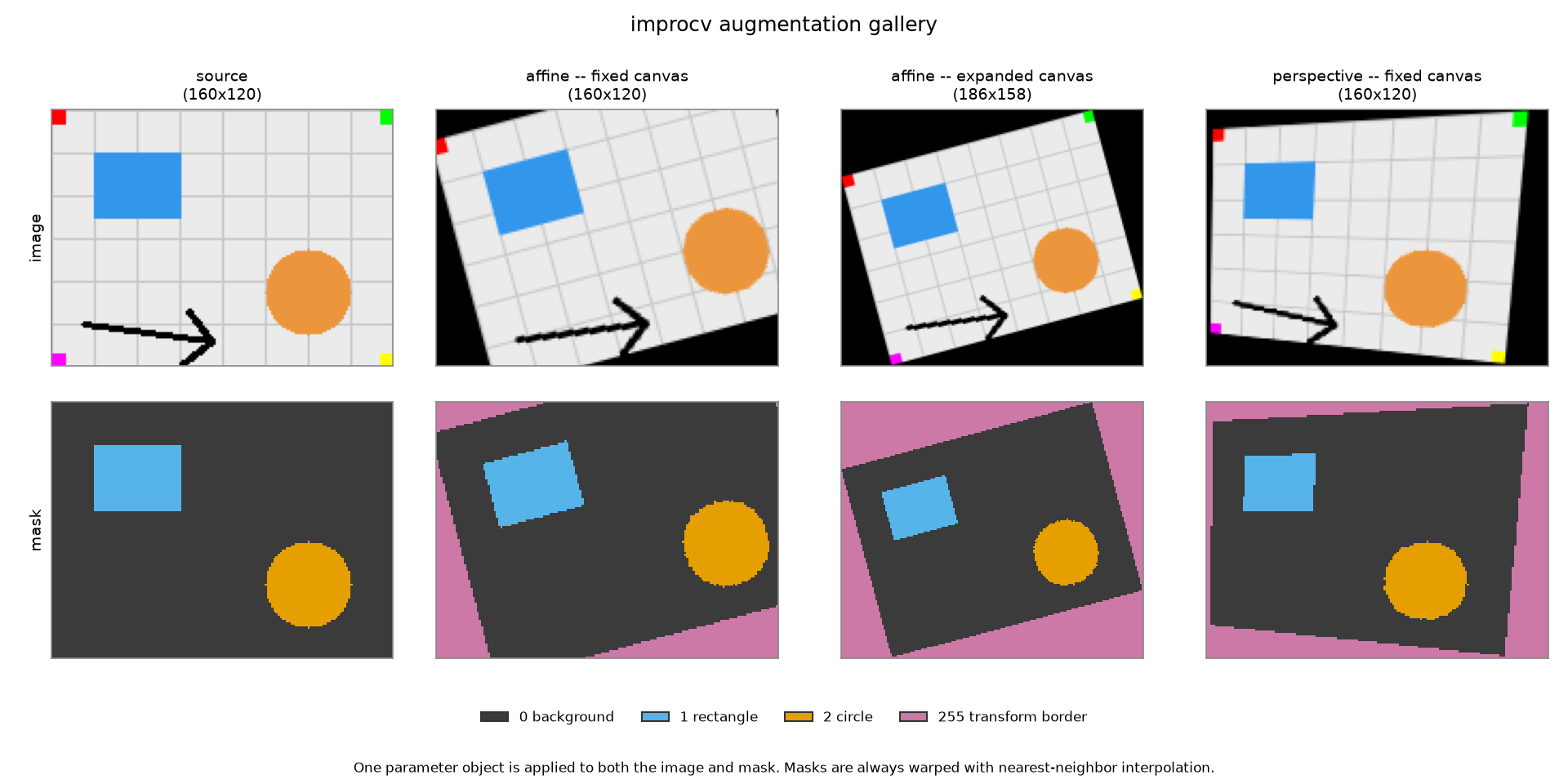
One sampled transform is applied to both the image and its mask, and the mask always keeps its original discrete labels (never an interpolated, illegal one). Affine transforms can render to a fixed canvas (content may be cropped) or an expanded one that grows to keep everything.

Regenerate this image and see other demos in demos/README.md.

Usage

import improcv as im

image = im.load_image("photo.jpg")
resized = im.resize(image, width=640)

load_image reads path's bytes through Python's own filesystem handling and decodes them with cv2.imdecode -- never cv2.imread(str(path), ...), whose filename-based handling is not reliable on Windows for paths containing characters outside the active code page. mode selects the decode policy:

image = im.load_image("photo.jpg")                      # mode="color" (default): BGR, uint8
gray = im.load_image("photo.jpg", mode="grayscale")      # 2-D, uint8, OpenCV's own gray decode
raw = im.load_image("image16.png", mode="unchanged")     # OpenCV's IMREAD_UNCHANGED result --
                                                           # dtype/channel count may vary by source

mode="grayscale" is OpenCV's own codec-level grayscale decode, not guaranteed identical to ensure_gray(im.load_image(path)). mode="unchanged" has no mask-specific semantics -- it is not a general segmentation-mask loader, and does not guarantee preserving a palette-indexed source as a class-index map. load_image reads a file's bytes exactly once and returns a new, independent array; see its docstring for the full path/error/decode contract.

Finding and sorting contours:

import cv2
import improcv as im

mask = im.threshold(im.ensure_gray(image), method="otsu")
contours, hierarchy = im.find_contours(mask, retrieval_mode="external")
contours, boxes = im.sort_contours(contours, order="left-to-right")

# `Contour` keeps OpenCV's own (N, 1, 2) int32 shape, so results pass
# straight into any cv2.* function that expects a contour — no conversion.
cv2.drawContours(image, contours, -1, (0, 255, 0), 2)

Connected components and flood fill:

import improcv as im

mask = im.threshold(im.ensure_gray(image), method="otsu")
num_labels, labels, stats, centroids = im.connected_components_with_stats(mask)
# stats[0]/centroids[0] describe the background label (0); inspect
# stats[label, 4] (area) before trusting a component's other statistics.

result = im.flood_fill(image, seed_point=(10, 10), new_value=(0, 255, 0))
print(result.filled_count, result.bounding_box)

Histogram and template matching:

import improcv as im

gray = im.ensure_gray(image)
hist = im.histogram(gray)  # channel=0, bins=256, value_range=(0.0, 256.0) by default

result = im.match_template(gray, template, method="ccoeff_normed")
match = im.min_max_loc(result)
print(match.max_loc)  # (x, y) of the best match

Segmentation and inpainting:

import improcv as im

markers = im.watershed(image, seed_markers)
# Positive values = regions, -1 = boundaries; 0 may remain unassigned.

foreground_mask = im.grabcut_rect(image, im.BoundingBox(x=20, y=20, width=200, height=150))

restored = im.inpaint(image, damage_mask, radius=3.0, method="telea")

Feature detection and description:

import cv2
import improcv as im

features = im.detect_and_compute(im.ensure_gray(image), method="orb")
print(len(features.keypoints), features.descriptors.shape, features.norm)

# features.keypoints are real cv2.KeyPoint objects -- pass them straight
# into any cv2.* function that expects them, no conversion needed.
annotated = cv2.drawKeypoints(image, features.keypoints, None)

Matching features between two images:

import cv2
import improcv as im

query = im.detect_and_compute(im.ensure_gray(image1), method="orb")
train = im.detect_and_compute(im.ensure_gray(image2), method="orb")

matches = im.match_features(query, train)
# matches is a plain list[cv2.DMatch], sorted by distance (best match
# first) -- pass it straight into cv2.drawMatches, no conversion needed.
annotated = cv2.drawMatches(image1, query.keypoints, image2, train.keypoints, matches, None)

# Or filter with Lowe's ratio test instead of match_features' cross-check:
ratio_matches = im.match_features_ratio(query, train, ratio=0.75)

# Estimate a RANSAC homography from the matches:
result = im.find_homography(query, train, ratio_matches)
if result.homography is not None:
    print(result.homography, result.inlier_mask.sum(), "inliers")

Hough transform shape detection:

import improcv as im

edges = im.auto_canny(im.ensure_gray(image))

lines = im.hough_lines(edges, threshold=100)
segments = im.hough_line_segments(edges, threshold=50, min_line_length=30, max_line_gap=10)

# hough_circles takes a grayscale image directly, not a binary edge mask.
circles = im.hough_circles(im.ensure_gray(image), min_dist=20, param2=30)
for circle in circles:
    print(circle.x, circle.y, circle.radius)

QR code decoding:

import improcv as im

code = im.decode_qr_code(image)
if code is not None:
    print(code.data, code.points)  # data is None if detected but undecodable

# For images that may contain more than one QR code:
for code in im.decode_qr_codes(image):
    print(code.data, code.points)

Barcode decoding (EAN-8, EAN-13, UPC-A):

import improcv as im

for barcode in im.decode_barcodes(image):
    print(barcode.data, barcode.barcode_type, barcode.points)
    # data/barcode_type are both None if detected but undecodable

Annotation drawing:

import improcv as im

mask = im.threshold(im.ensure_gray(image), method="otsu")
contours, _ = im.find_contours(mask)
boxes = im.bounding_boxes(contours)

annotated = im.draw_contours(image, contours, color=(0, 255, 0), thickness=2)
annotated = im.draw_bounding_boxes(annotated, boxes, color=(255, 0, 0), thickness=2)
# Both return a new array; `image` itself is never modified.

# Tiling several images into one grid:
grid = im.montage([image, annotated], tile_width=200, tile_height=200)

Point/region detectors:

import cv2
import improcv as im

gray = im.ensure_gray(image)

fast_keypoints = im.detect_fast_keypoints(gray)
blob_keypoints = im.detect_blob_keypoints(gray)
annotated = cv2.drawKeypoints(image, fast_keypoints, None)
annotated = cv2.drawKeypoints(annotated, blob_keypoints, None)

mser_regions = im.detect_mser_regions(gray)
# region.points is every pixel belonging to the region as an unordered
# set -- not an ordered boundary, so don't pass it to draw_contours.
# Use the region's bounding box instead:
annotated = im.draw_bounding_boxes(annotated, [region.bounding_box for region in mser_regions])

Visualization (optional, requires pip install "improcv[viz]"):

import improcv.visualization as viz

viz.show_image(image, title="input")  # handles BGR->RGB, hides axes by default
viz.plot_histogram(image)              # one line per channel (B/G/R or grayscale)

Image quality metrics:

import improcv as im

error = im.mse(original, compressed)
quality_db = im.psnr(original, compressed)      # math.inf if the images are identical
similarity = im.ssim(original, compressed)      # 1.0 for identical images, not clamped otherwise

# float images need an explicit data_range; uint8 and uint16 infer it automatically:
similarity = im.ssim(original_f32, compressed_f32, data_range=1.0)

# gmsd is grayscale-only (2D, or 3D with exactly 1 channel) -- convert first
# with im.ensure_gray. Unlike ssim/psnr, lower is better: 0.0 for identical
# images; higher values generally indicate greater distortion according to
# GMSD.
distortion = im.gmsd(im.ensure_gray(original), im.ensure_gray(compressed))

Perceptual hashing:

import improcv as im

# uint8 only: grayscale (H, W)/(H, W, 1), BGR (H, W, 3), or BGRA (H, W, 4).
# For color input, alpha (if present) is ignored, not composited.
a = im.average_hash(original)
b = im.phash(compressed)              # a different algorithm -- see below
c = im.phash(compressed_but_blurred)

distance = c.distance(im.phash(compressed))    # Hamming distance, an int -- lower means more similar
print(c)                                       # fixed-width, lowercase hex

# a.distance(b) would raise ValueError: average_hash and phash are different,
# non-comparable algorithms even though both produce 64-bit hashes by default.

# round-tripping through hex requires the algorithm and hash_size explicitly --
# a hex string alone can't reveal which algorithm produced it:
restored = im.PerceptualHash.from_hex(str(c), algorithm=im.PerceptualHashAlgorithm.PHASH)
assert restored == c

A perceptual hash is not a cryptographic one: collisions are expected, and a smaller Hamming distance usually (not always) means more visually similar images. average_hash/phash reproduce cv2.img_hash's own bit decisions for hash_size=8 -- but not its packed-byte serialization, and not other libraries' (e.g. ImageHash) genuinely different, incompatible variants of the same algorithm names.

Dataset image similarity:

import improcv as im

manifest = im.build_perceptual_hash_manifest(
    "images",
    algorithm=im.PerceptualHashAlgorithm.PHASH,
    hash_size=8,
)

pairs = im.find_similar_image_pairs(
    manifest.to_hashes(),
    max_distance=8,
)

for pair in pairs:
    print(pair.distance, pair.first, pair.second)

This no longer needs from pathlib import Path or import cv2: build_perceptual_hash_manifest discovers every image under "images" with discover_images (inheriting its own ordering, symlink, hidden-file, and extension-matching rules unchanged), decodes each one exactly once as fixed 8-bit grayscale, and hashes it with the requested algorithm -- all in one call, never using cv2.imread. Each resulting identifier is relative to "images" itself; "images" is never stored as a segment of any entry path, so renaming that directory later doesn't change what the manifest says about the files inside it (see "A real bug this fixes" below). The first file whose bytes can't be decoded as an image raises ValueError immediately, naming that file; a native error reading a file's bytes at all (missing file, permission denied, or another filesystem error) propagates unchanged instead, since that's a different failure mode from an undecodable image. Like the manual pipeline it replaces, the builder only ever returns a PerceptualHashManifest -- it does not save it (see persistence below), it is not a cache, it does not check freshness, and it does not run any work in parallel.

find_similar_image_pairs never touches the filesystem, decodes an image, or computes a hash itself -- it only compares the PerceptualHash values you already have, once per unordered pair. That separation means hashes are computed exactly once, and the same collection can be re-searched at a different max_distance without redecoding or rehashing anything. The threshold has no library-provided default and must be chosen for your own application and algorithm. The result is a tuple of matching pairs, not duplicate groups: threshold similarity is not transitive (A close to B and B close to C does not imply A close to C), so pairs are reported independently rather than merged into clusters. Comparing every pair costs O(n**2) -- this first slice is a simple, deterministic building block, not a promise to scale to millions of images.

A real bug this fixes: an earlier version of this README built the hash mapping by hand, keyed by the root-anchored path discover_images returns (hashes[path] = im.phash(image)), then handed that mapping straight to PerceptualHashManifest.from_hashes. discover_images preserves whichever form its root argument had -- a relative root like "images" (the snippet's own root) yields root-anchored relative paths such as Path("images/cat.jpg"), not absolute ones; only an absolute root (e.g. Path("/datasets/images")) yields absolute results. So the earlier mapping's keys were never absolute paths -- but Path("images/cat.jpg") still isn't the same thing as a true dataset-root-relative identifier: it still carries the "images" root segment, where path.relative_to("images") would give the actual root-relative path, Path("cat.jpg"). from_hashes stores whatever path it's given as-is -- it has no notion of a "dataset root" to relativize against, so it cannot strip that root prefix for you -- so keys built that way became manifest identifiers like images/cat.jpg, not cat.jpg. That's a real, working relative path, but it silently embeds the old root directory's own name; rename images/ to photos/ later and every stored identifier is now wrong relative to the new layout, even though nothing about the images themselves changed. build_perceptual_hash_manifest fixes this structurally, not by convention: it relativizes every discovered path against the exact root you passed it ("images" above, via path.relative_to(root)), so identifiers are always cat.jpg, never images/cat.jpg, regardless of what the root directory happens to be named.

A complete runnable recipe using the builder is available in examples/dataset_manifest_builder.py -- a concise builder-based workflow covering discovery, decoding, hashing, persistence, moving the dataset root, and a similarity search, entirely through public API.

A second recipe, examples/image_similarity.py, demonstrates hashes, distances, and non-transitivity specifically -- not the builder -- calling discover_images and average_hash directly on hand-checkable synthetic images.

<img src="https://raw.githubusercontent.com/michalmaj/improcv/main/docs/assets/image-similarity-gallery.png" alt="improcv image similarity showing four synthetic 8x8 images with their average_hash hex values, a symmetric 4x4 Hamming distance matrix with two in-threshold pairs highlighted, and the two pairs returned by find_similar_image_pairs at max_distance=2 with a_base.png and c_variant_more.png shown as a non-transitive gap at distance 4" width="880"

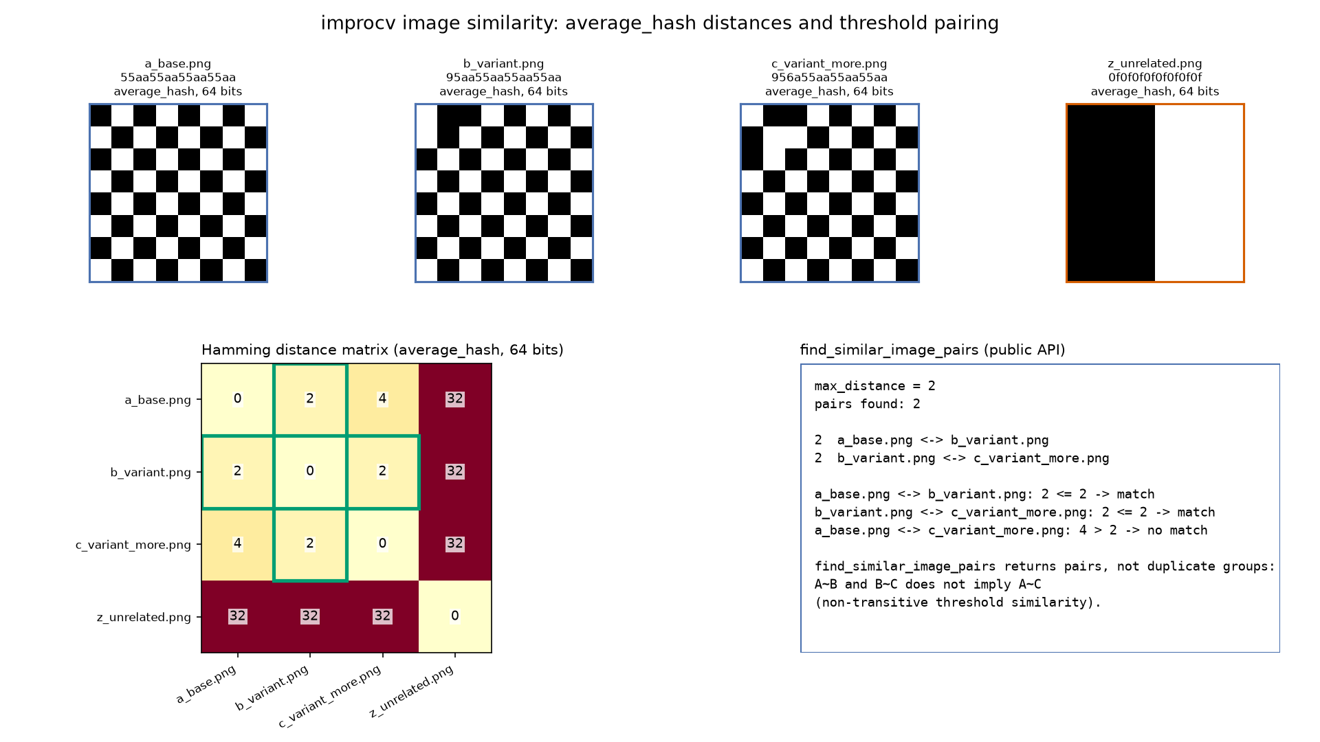
The image is generated by demos/image_similarity_gallery.py, which uses average_hash on four small, hand-checkable synthetic images (rather than phash, as in the snippet above) specifically to make its exact hash bits and Hamming distances verifiable, and to show find_similar_image_pairs reporting a non-transitive pair of matches -- both are intentionally correct, complementary illustrations of the same API, not a contradiction.

Precomputed hashes don't have to be recomputed every run: PerceptualHashManifest (the manifest already built above) snapshots a path -> PerceptualHash mapping as deterministic JSON, so the same hashes can be saved once and reused later, or shared with another machine:

manifest.save("image-hashes.json")

restored = im.PerceptualHashManifest.load(
    "image-hashes.json"
)

pairs = im.find_similar_image_pairs(
    restored.to_hashes(),
    max_distance=8,
)

There's no need to rebuild the manifest with PerceptualHashManifest.from_hashes(...) here -- the builder above already returned one. from_hashes is what you'd reach for only if you had a path -> PerceptualHash mapping from somewhere other than the builder; it has no notion of a dataset root, so it cannot make a manually keyed mapping relative to one for you -- a mapping keyed by paths that still include the old root directory's name stays exactly that way, not just a "relative path" in some looser, still-portable sense. build_perceptual_hash_manifest's identifiers are relative to the dataset root itself, by construction, which is the actual portability guarantee (see "A real bug this fixes" above) -- not merely relative paths that may still embed the old root's directory name.

A manifest stores each path as a portable, relative, POSIX-style identifier -- never an absolute path -- so the same JSON is valid regardless of which machine or directory it was built on, and to_json()/from_json() (and, in turn, save()/load()) round-trip byte-for-byte regardless of the input mapping's insertion order. save() writes UTF-8, deterministic JSON text and publishes it atomically; by default (overwrite=False) it never clobbers an existing file at that path -- saving again under the same name requires manifest.save(path, overwrite=True) explicitly. The parent directory is never created automatically. It is still a snapshot, not a cache: save/load add a file transport, nothing else -- the manifest never checks whether a path still exists, never checks freshness, never records file size or modification time, and keeping it in sync with the images it describes is entirely the caller's responsibility. to_json()/from_json() remain available for in-memory transport (e.g. sending a manifest over a network) when a file isn't wanted at all.

A complete runnable persistence workflow using the builder is available in examples/dataset_manifest_builder.py. A second, manual step-by-step equivalent -- showing explicit discovery, decoding, hashing, relative_to(root), and from_hashes -- is available in examples/image_similarity_manifest.py.

Comparing two manifests of the same logical dataset from different points in time:

diff = im.compare_perceptual_hash_manifests(before, after)

print(len(diff.added), len(diff.removed), len(diff.changed), len(diff.unchanged))
for change in diff.changed:
    print(change.path, change.before, "->", change.after)

compare_perceptual_hash_manifests classifies every path in before/after by canonical manifest path identity alone: a path present only in after is added, present only in before is removed, present in both with a different hash is changed, and present in both with an identical hash is unchanged -- diff.added/diff.removed are full PerceptualHashManifestEntry values, diff.changed is a tuple of PerceptualHashManifestChange (path plus the hash on each side), and diff.unchanged is a tuple of bare paths. A rename is always reported as one removed entry plus one added entry, never specially detected or merged -- even when the hash under the old and new path is identical. An identical hash under different paths does not establish that a rename occurred: it may represent renamed content, duplicated content, perceptually similar content, or a hash collision (see improcv.hashing for why perceptual hash collisions are expected, not a defect). compare_perceptual_hash_manifests deliberately does not infer which case occurred -- path identity remains the only identity rule, so the result is always removed+added. before/after must share the same algorithm and hash_size, or this raises ValueError, exactly like PerceptualHash.distance and find_similar_image_pairs already require of their own inputs. This function performs no filesystem access and no image decoding -- it only compares two already-constructed PerceptualHashManifest values in memory, so it works identically whether they came from build_perceptual_hash_manifest, PerceptualHashManifest.load, or from_hashes. Like the manifest itself, this is a snapshot comparison, not a cache or a freshness check: it says nothing about whether either manifest is still valid against the current contents of the dataset it describes. This is a separate operation from find_similar_image_pairs: comparing two manifests is path-identity based and has nothing to do with perceptual similarity between images, and compare_perceptual_hash_manifests never calls it.

A complete runnable example is available in examples/manifest_comparison.py.

Photo/creative single-image effects:

import improcv as im

# uint8 only, exactly 3-channel BGR -- no automatic grayscale/BGRA handling.
bgr = im.ensure_bgr(gray)          # convert grayscale first if needed
sketch = im.pencil_sketch(bgr)     # sketch.grayscale: (H, W); sketch.color: (H, W, 3)
stylized = im.stylize(bgr)
enhanced = im.detail_enhance(bgr)

# BGRA must be handled explicitly before calling -- ensure_bgr does not
# accept it, since there's no single correct way to turn alpha into BGR:
bgr_from_bgra = bgra[..., :3]                    # drop alpha, or
# bgr_from_bgra = your_own_alpha_compositing(bgra)  # composite onto a background

sigma_s/sigma_r (and pencil_sketch's shade_factor) are restricted to the ranges OpenCV's own API documents (0 < sigma_s <= 200, 0 < sigma_r <= 1, 0 <= shade_factor <= 0.1) -- verified directly that sigma_r=0 leads to division by zero internally, and that values beyond these ranges are unsupported by OpenCV's own contract (the parameters are stored as a C++ float, so extreme values can silently degrade to a useless result).

Seamless cloning (Poisson image editing):

import improcv as im

result = im.seamless_clone(
    source,
    destination,
    mask,
    center=(x, y),
    mode="normal",
)

source/destination are uint8 BGR (H, W, 3) -- no automatic conversion, and they don't need to be the same size. mask is a uint8 (H, W) array matching source's spatial size, with only 0/255 accepted. OpenCV always ignores mask's outermost 1-pixel border, and the bounding box of what remains (after that border is zeroed) must be at least 3x3 pixels. center=(x, y) is in destination's coordinate system and is where that bounding box's center is placed -- not the center of all of source or all of mask. There is no automatic alpha handling. Seamless cloning reconstructs the pasted region from gradients, not by copying pixels -- so a flat-colored source region can produce little or no visible change, unlike the "cut and paste" effect of alpha blending. "mixed" picks whichever of source's/destination's gradient is stronger at each pixel (useful for loosely-drawn masks); "monochrome_transfer" transfers source's luminance structure rather than its color. The result always has destination's shape and dtype.

HDR-related operations (improcv.hdr) are split into distinct techniques, not one "HDR" feature: Mertens exposure fusion directly combines aligned LDR images into a display-oriented float32 result without reconstructing physical radiance; radiance HDR merge reconstructs an actual HDR radiance map from a stack plus its exposure times; camera-response calibration estimates the response curve that merge can use instead of its default fixed linear one; tone mapping then compresses that radiance map's dynamic range back down for display. All four are implemented below.

Exposure fusion:

import numpy as np
import improcv as im

fused = im.fuse_exposures(images)  # images: list/tuple of uint8, same shape, at least 2

# fused is float32, nominally close to [0, 1] but not clipped to it --
# convert explicitly before saving/displaying as uint8:
display = np.clip(fused, 0.0, 1.0)
display_u8 = np.round(display * 255.0).astype(np.uint8)

fuse_exposures wraps OpenCV's Mertens exposure fusion: it blends the stack directly (in the domain of a Laplacian pyramid, weighted by local contrast/saturation/well-exposedness), producing a single well-exposed image -- it does not need exposure times and does not produce a physical HDR radiance map, so its result does not need (and should not go through) tone mapping. images must be a real Sequence (list/tuple, or another collections.abc.Sequence) of at least 2 uint8 images, either all 2D grayscale or all 3D BGR (H, W, 3) with identical shape -- a single stacked array, (H, W, 1), 2-channel, and BGRA are all rejected, with no automatic conversion. contrast_weight/ saturation_weight/exposure_weight must be non-negative and finite; 0 is legal for all three (it's exposure_weight's own default). Repeated calls with identical input are not guaranteed to be bit-for-bit identical -- OpenCV's implementation uses internal parallel summation.

Radiance HDR merge -- without calibration (OpenCV's fixed linear response):

import improcv as im

hdr = im.merge_hdr_debevec(images, exposure_times)  # or im.merge_hdr_robertson(...)

With a calibrated response curve:

response = im.calibrate_camera_response_debevec(images, exposure_times)
hdr = im.merge_hdr_debevec(images, exposure_times, response_curve=response)

# or the Robertson equivalent:
response = im.calibrate_camera_response_robertson(images, exposure_times)
hdr = im.merge_hdr_robertson(images, exposure_times, response_curve=response)

images[i] and exposure_times[i] are paired by index -- neither is ever reordered. All exposure times must use one consistent unit (conventionally seconds): uniformly rescaling every time by a constant factor rescales the entire output radiance map by the reciprocal of that factor. Not passing response_curve does not calibrate anything -- calibration is always an explicit, separate step you call yourself; OpenCV uses a fixed linear response instead if you don't. The output is a raw radiance map (float32, typically ranging far beyond [0, 1], not clipped or normalized) -- it is not display-ready and needs tone mapping (see below) before it can be saved or shown; do not write it directly as a uint8 image. Both merge functions accept BGR only -- grayscale is not supported by either. merge_hdr_robertson raises a raw cv2.error for grayscale regardless of dtype, verified directly. merge_hdr_debevec's own default (no explicit response_curve) linear-response construction has a confirmed bug in OpenCV's own C++ source that corrupts memory for a genuinely 1-channel array -- undefined behavior that happens not to crash on some platforms but crashed the process outright (a non-catchable native abort) in this project's own CI on another, so grayscale is rejected unconditionally for both merge functions rather than only in the specific triggering case. uint8, uint16, and float32 are all accepted for BGR merge (float32 values must be finite and within [0, 1]). uint16/float32 additionally require an OpenCV build that supports them for HDR merge -- verified directly that OpenCV 4.9.0 (this project's documented minimum) only supports uint8 here; a clear ValueError is raised instead of a raw OpenCV error on an older build. Calibration itself is always uint8-only (for both algorithms), so its output is always a 256-entry curve -- it pairs directly with a uint8 merge, not automatically with a uint16/float32 one. calibrate_camera_response_debevec accepts grayscale or BGR; calibrate_camera_response_robertson is BGR only (raises a clear error pointing at the Debevec calibrator for a grayscale stack). calibrate_camera_response_debevec's random_sampling=True samples pixel locations randomly with no seed control in OpenCV's own API -- its result is not guaranteed reproducible across calls. calibrate_camera_response_robertson needs a reasonably diverse intensity histogram to produce a finite curve at all: verified directly that an all-black or all-white image stack (or one with very few distinct intensity values) deterministically raises RuntimeError here, regardless of image size. calibrate_camera_response_debevec is generally more robust to sparse or degenerate intensity histograms because of its smoothness regularization, but a finite result is not guaranteed on every supported OpenCV build. Non-finite or otherwise merge-incompatible curves raise RuntimeError. Neither calibrator performs exposure alignment or ghost removal -- the input stack is assumed already aligned, for both calibration and merge.

Tone mapping -- compressing a radiance map down to a display-ready image:

import numpy as np
import improcv as im

response = im.calibrate_camera_response_debevec(images, exposure_times)
hdr = im.merge_hdr_debevec(
    images,
    exposure_times,
    response_curve=response,
)
tone_mapped = im.tone_map_reinhard(hdr)

display_u8 = np.round(
    np.clip(tone_mapped, 0.0, 1.0) * 255.0
).astype(np.uint8)

A radiance map from merge_hdr_debevec/merge_hdr_robertson is not display-ready -- its values typically extend far beyond [0, 1] and are not clipped or normalized. Tone mapping compresses that dynamic range back down to something a display or uint8 file can represent. Four operators are provided, wrapping OpenCV's own cv2.createTonemap/createTonemapDrago/createTonemapReinhard/ createTonemapMantiuk: tone_map (simple linear normalization with gamma correction), tone_map_drago (adaptive logarithmic compression), tone_map_reinhard (photographic, local/global adaptation blend), and tone_map_mantiuk (contrast-domain compression via an iterative solver -- markedly more expensive than the other three). Each has its own parameters and produces a visibly different look; none is a drop-in replacement for another. All four return raw float32 -- none of them clip, normalize, or quantize their output, even though OpenCV's own documentation describes the result as [0, 1]: verified directly that a spatially constant input (e.g. a flat, saturated region) can produce output well outside that range. Always clip explicitly (np.clip(..., 0.0, 1.0)) before converting to uint8, as in the example above. hdr must be float32, shape (H, W, 3) (BGR -- tone mapping never converts to RGB), finite, and non-empty for all four functions; negative values are allowed, since neither merge function guarantees non-negative radiance. tone_map_reinhard and tone_map_mantiuk additionally reject a spatially constant hdr (ValueError) -- verified directly, in OpenCV's own C++ source, that both divide by a quantity that is exactly zero for a constant image, regardless of parameters. tone_map_drago and tone_map_mantiuk additionally reject an hdr that would produce a true zero-luminance (black) pixel once run through OpenCV's own internal normalization -- a common case, not just a synthetic one (any hdr whose darkest point across all three channels is a true black pixel triggers it). tone_map_mantiuk additionally requires both hdr dimensions to be at least 2. See each function's docstring for the full parameter contract and exact value ranges.

A finite result is not unconditionally guaranteed even for well-formed, non-degenerate hdr. All four operators internally raise a normalized value to some exponent (gamma, tone_map_drago's bias, or an internal, non-parametrized exponent for tone_map_reinhard/tone_map_mantiuk); OpenCV's own floating-point rounding can occasionally leave that value very slightly negative -- an ordinary artifact of min/max normalization, not a data problem -- and raising a negative number to a non-integer power is mathematically undefined, producing NaN. Whether this actually happens is CPU-architecture/SIMD-dispatch-dependent, not just data-dependent: verified directly that the same seed and parameters that tone-map finitely on Apple Silicon produced a non-finite result (cleanly caught by RuntimeError) on x86_64 CI. Treat RuntimeError from any tone-mapping function as a real, expected possibility for otherwise-ordinary input, not only for the degenerate cases listed above.

Mertens exposure fusion (fuse_exposures, above) is a different operation and does not produce a radiance map -- do not run its output through any of the tone-mapping functions; its result is already close to display-ready (see its own section above).

Non-local means denoising:

import improcv as im

denoised = im.nl_means_denoise(gray)                # uint8 2D grayscale
denoised_bgr = im.nl_means_denoise_colored(bgr)      # uint8 (H, W, 3) BGR

Both are uint8-only with no automatic conversion (grayscale/BGR/BGRA/2-channel input to the wrong function is rejected, not silently handled). Higher h (and h_color for the colored version) generally smooths more aggressively but can also remove real detail. nl_means_denoise_colored works internally in CIELAB (denoising luminance and color separately, like OpenCV's own implementation) -- unlike the grayscale version, h_luminance=0, h_color=0 does not guarantee a result identical to the input, since the BGR/CIELAB round-trip alone can shift values slightly. Larger search_window_size values can substantially increase execution time; 7/21 (template_window_size/search_window_size) are OpenCV's own recommended defaults, not hard limits. template_window_size and search_window_size are independent parameters -- there is no requirement that search_window_size be at least template_window_size.

Panorama and scan stitching:

import improcv as im

panorama = im.stitch_images(
    images,
    mode="panorama",
)

# flat scans / documents captured under a simpler planar transformation:
scan = im.stitch_images(images, mode="scans")

stitch_images wraps OpenCV's high-level cv2.Stitcher. images must be a real Sequence (list, tuple, or another collections.abc.Sequence) of at least 2 uint8 BGR (H, W, 3) images -- a single stacked array (including 4D), str/bytes/bytearray, and a generator/iterator are all rejected explicitly, as are grayscale, (H, W, 1), 2-channel, BGRA, uint16, float32, and float64 images, with no automatic conversion. Images may have different spatial shapes -- there is no requirement that they match. mode="panorama" (the default) uses a homography/perspective model, suited to photos taken by rotating a camera; mode="scans" uses an affine model, suited to flat scans or documents -- "scans" is not limited to pure translational sliding, it is a broader affine model, just not projective/perspective. Both modes share the identical input/output contract.

On success, the result is a new, independent uint8 BGR array -- not cropped, and not guaranteed any particular shape, aspect ratio, or relationship to the input sizes. Insufficient overlap, too few usable features, or an algorithmic failure of homography/camera-parameter estimation all raise RuntimeError (never ValueError -- the input images are structurally fine, the algorithm simply could not relate them), naming the specific OpenCV status and its numeric code.

Neither the outcome nor the exact result is guaranteed deterministic, even within a single process. OpenCV's feature matching and geometry estimation use RANSAC internally, drawing from OpenCV's global RNG -- verified directly that, for a borderline amount of overlap, the same input images can succeed on one call and fail with RuntimeError on the next, in the same process, and that even a reliably successful stitch is not guaranteed to produce the same output shape or pixel values across repeated calls. stitch_images never calls cv2.setRNGSeed itself -- that would silently change OpenCV's global RNG state for every other OpenCV call in the process, not just this one. You can call cv2.setRNGSeed yourself before calling stitch_images if reproducibility matters for your own experiments, but that is a process-global setting, not a per-call one, and it does not promise identical results across different OpenCV builds or platforms.

Stitching can be expensive in both time and memory, in a way this wrapper cannot safely bound. OpenCV allocates the output panorama and its internal intermediate buffers inside stitch(), before control returns to Python -- verified directly that a poorly-conditioned geometry estimate (e.g. two images whose relative orientation does not match what mode expects) can make OpenCV allocate, and report as a successful result, a panorama and intermediate buffers many times larger than the inputs. Because the large allocation already happens before this wrapper ever sees a return value, no check on the returned array could have prevented it, so stitch_images does not attempt one. For untrusted or unpredictable input sets, consider running this function in an isolated process with its own resource limits, or use OpenCV's lower-level stitching pipeline directly for finer control.

Per-image feature masks supported by the lower-level OpenCV Stitcher API are not exposed by this wrapper. This first version also does not expose any of cv2.Stitcher's registration/seam/ compositing/confidence settings -- it always uses OpenCV's own defaults.

DNN preprocessing:

import improcv as im

blob = im.create_dnn_blob(
    image,
    size=(224, 224),
    scale=1.0 / 255.0,
    mean=(0.0, 0.0, 0.0),
    swap_rb=True,
)

# a batch of images sharing one set of parameters:
batch = im.create_dnn_batch_blob(
    [image_a, image_b],
    size=(224, 224),
    scale=1.0 / 255.0,
    swap_rb=True,
)

create_dnn_blob/create_dnn_batch_blob wrap cv2.dnn.blobFromImage/blobFromImages to turn a uint8/float32 image (or a Sequence of them) into a blob ready for cv2.dnn.Net.setInput -- they do not load a model, create a cv2.dnn.Net, or run inference; that is a separate, later slice. The output is always float32 and always 4-D NCHW ((1, C, H, W) for a single image, (N, C, H, W) for a batch) -- a single image still gets an explicit batch dimension, there is no 3-D HWC return path. size is (width, height), matching OpenCV's own convention, not NumPy's (height, width) indexing order. crop=False (the default) resizes directly to size, stretching independently in each dimension without preserving aspect ratio; crop=True uniformly scales the image so it covers size in both dimensions, then takes a centered crop -- both always use OpenCV's INTER_LINEAR, which is not configurable, because the underlying OpenCV function does not expose an interpolation parameter either.

The operation is (input - mean) * scale. A scalar mean (e.g. mean=1.0) is broadcast by improcv to every channel; passing that same scalar directly to raw cv2.dnn.blobFromImage would not broadcast it -- it would be interpreted as only the first channel's mean, leaving the others at zero. A tuple mean must have exactly one element per channel, and its order refers to the output channel order: for BGR/BGRA input, swap_rb=False means (B, G, R[, A]) and swap_rb=True means (R, G, B[, A]) -- passing BGR-ordered image data does not, by itself, produce RGB-ordered output; swap_rb=True is required for that, and it never touches an alpha channel, which always stays last.

create_dnn_batch_blob requires an explicit size -- there is no "keep native size" default for a batch, because OpenCV silently resizes every image after the first to match the first image's native size when no size is given, which silently produces wrong results for a batch of differently-sized images. create_dnn_blob (single image) does default size to None, which keeps that one image's native size.

Only uint8 and float32 input is accepted (grayscale, (H, W, 1), BGR, or BGRA) -- verified directly that other dtypes accepted by raw OpenCV on some versions (e.g. int16, uint16, float64) are silently converted on OpenCV >= 4.13 but raise a raw cv2.error on OpenCV 4.9, so allowing them here would make behavior depend on the installed OpenCV version. There is no output_dtype parameter in this first version -- the output is always float32; a uint8-output mode may be added later, compatibly, as a new keyword-only parameter if a concrete need for it appears.

Extremely large size values can exhaust process memory or be killed by the operating system -- this is not, and cannot be, turned into a catchable Python exception. size is validated to be representable (each dimension and their product must fit a signed 32-bit int, matching an internal limit in OpenCV's own blob-construction code), but that says nothing about whether the resulting allocation is a reasonable size for the machine running it -- pick size based on your actual model input requirements, not arbitrarily large values.

No DNN inference or cv2.dnn.Net configuration (backend/target) is included in this slice, and no new dependency (or improcv[ml] extra) was introduced for it -- both functions run on the same base OpenCV install as the rest of improcv. ONNX model loading is implemented below as a separate Phase 5 slice.

ONNX model loading:

import improcv as im

net = im.load_onnx_network("model.onnx")

blob = im.create_dnn_blob(
    image,
    size=(224, 224),
    scale=1.0 / 255.0,
    swap_rb=True,
)

net.setInput(blob)
output = net.forward()

load_onnx_network/load_onnx_network_from_bytes load an ONNX file (from a path or from an in-memory bytes buffer, respectively) into a cv2.dnn.Net -- they are ONNX-only, not a generic "load any DNN model" function; other formats (TensorFlow, Caffe, Darknet, Torch, OpenVINO) are out of scope. Preprocessing (create_dnn_blob/create_dnn_batch_blob, above) and model loading are both improcv API; Net.setInput/Net.forward (shown above) remain raw OpenCV API, not wrapped -- this slice does not add an inference function, model-specific postprocessing, or a backend/target API.

The path and bytes loaders are two separate functions, not one function accepting either, because a bare bytes argument is genuinely ambiguous to raw OpenCV: verified directly that cv2.dnn.readNetFromONNX(some_bytes) (positional) is silently routed to the path overload on OpenCV 4.13/5.0 (interpreting the bytes as a file path and failing to find it) but to the buffer overload on OpenCV 4.9 -- an actual behavioral difference between supported versions, not a hypothetical one. load_onnx_network_from_bytes only accepts bytes (not bytearray, memoryview, or an ndarray) and internally converts to a uint8 array before calling OpenCV by keyword, which resolves correctly and identically on every supported version.

load_onnx_network's path accepts a str or os.PathLike[str] (e.g. pathlib.Path); its content, not its extension, is what's parsed -- a valid ONNX file with no .onnx extension is accepted. Filesystem problems that Python can detect directly give native exceptions (FileNotFoundError, IsADirectoryError, an empty file raises ValueError); a problem OpenCV's own parser hits (a corrupt/invalid model, or a permission/ACL issue that only surfaces once OpenCV tries to open the file) raises RuntimeError with the original error attached as __cause__. A path containing non-ASCII characters is not guaranteed to work identically on every platform -- verified directly (via CI) that the same accented path opens fine on Linux/macOS but makes OpenCV's own file-opening code fail on Windows (surfacing as RuntimeError, not a bug in this wrapper's validation); prefer an ASCII-only path where cross-platform behavior matters.

Every call to either loader parses the model again and returns a new, independent cv2.dnn.Net -- nothing is cached, and repeated loading of a large model is exactly as expensive as it looks. The returned Net is a stateful object: calling setInput() mutates it, backend/target configuration is your responsibility, and this wrapper makes no thread-safety promise about it.

On OpenCV 5, improcv requests ENGINE_CLASSIC as the common behavior shared with OpenCV 4.x, since 4.x has no other engine. OpenCV process configuration, including OPENCV_FORCE_DNN_ENGINE, may override that request -- this is a best-effort request, not a guarantee.

ONNX models are parsed by OpenCV's native (C++) code, with no sandboxing from this wrapper. There is no file-size limit, and no attempt is made to validate the ONNX format beyond what OpenCV's own parser does. A malicious or merely corrupted model can exploit a parser bug, and a very large model can consume a large amount of memory or end the process outright -- the same risk as parsing any untrusted binary format. Do not load models from untrusted sources in-process; isolate them in a separate process with its own resource limits instead. This slice does not download models from anywhere -- you provide the path or bytes.

Classification evaluation:

import improcv as im

cm = im.confusion_matrix(
    y_true=[0, 0, 1, 1],
    y_pred=[0, 1, 1, 1],
    labels=[0, 1],
)

metrics = im.classification_metrics(
    y_true=[0, 0, 1, 1],
    y_pred=[0, 1, 1, 1],
    labels=[0, 1],
    average=None,
)

# both accept an optional, keyword-only sample_weight too
weighted_cm = im.confusion_matrix(
    y_true=[0, 0, 1, 1],
    y_pred=[0, 1, 1, 1],
    labels=[0, 1],
    sample_weight=[2.0, 1.0, 3.0, 4.0],
)

confusion_matrix/classification_metrics cover single-label multiclass classification with integer labels only -- one true class and one predicted class per sample, not multilabel, and not string/hashable labels. cm.matrix[i, j] counts samples whose true class is cm.labels[i] and predicted class is cm.labels[j]: rows are true labels, columns are predicted labels. labels=None infers the class universe as the sorted union of every value observed in y_true/ y_pred; an explicit labels fixes the exact row/column order instead. improcv raises ValueError in two cases where sklearn.metrics.confusion_matrix does not: a duplicate value within an explicit labels (sklearn silently accepts it, but with confusing index semantics -- the repeated label's row/column gets written to by whichever occurrence's index NumPy resolves last, not merged or rejected), and an observed y_true/y_pred value outside an explicit labels (sklearn silently drops that sample from the matrix instead of erroring).

classification_metrics's result type depends on average: average=None (the default) gives precision/recall/f1 as per-class, read-only float64 arrays; average="micro"/"macro"/ "weighted" gives them as plain Python floats instead -- never both forms from the same call. support is always a per-class, read-only array regardless of average (int64/float64 per the sample_weight rule below), and accuracy is always a plain float. zero_division (0.0, 1.0, or "nan") controls what a class reports when its own division is genuinely undefined -- precision, recall, and F1 each have their own zero-division condition, checked independently from true positive/false positive/false negative counts (TP/FP/FN), never from each other: precision uses zero_division only when TP + FP == 0 (the class was never predicted); recall uses it only when TP + FN == 0 (the class never occurs in the true labels); F1 uses it only when 2*TP + FP + FN == 0 (the class is completely absent from both). A class with TP = 0 but real, nonzero FP/FN has a correctly defined F1 = 0 -- zero_division does not turn that 0 into 1.0 or NaN. With "nan", an actually-undefined value's NaN propagates into "macro"/"weighted" aggregates by plain averaging, not by skipping the affected class, including when that class's own support (and therefore its weight) is zero.

A confusion matrix already computed (including one you've aggregated yourself from several batches, e.g. ConfusionMatrixResult(matrix=sum(batch_matrices), labels=original_labels)) can be passed to classification_metrics_from_confusion_matrix directly, without recomputing it from raw labels -- since such a matrix is never re-derived from y_true/y_pred, its total count is verified to fit in int64 before support/precision/recall/F1 are computed, raising ValueError instead of silently wrapping around to a negative count if it doesn't. An empty confusion matrix is possible only with explicit labels (confusion_matrix([], [], labels=[0, 1]) returns a well-defined all-zero matrix); classification_metrics, classification_metrics_from_confusion_matrix, and confusion_matrix with labels=None all require at least one observation. Building the dense matrix costs O(len(labels) ** 2) memory, so a very large explicit labels can exhaust process memory even though improcv checks the allocation is at least representable first.

confusion_matrix/classification_metrics both accept an optional, keyword-only sample_weight (None by default). ConfusionMatrixResult.matrix/ClassificationMetrics.support are exactly int64 when sample_weight was not given, exactly float64 whenever it was -- even sample_weight=[1.0, ...] or an all-integer weight sequence, regardless of the weights' own dtype or values; dtype alone carries this information, so equality (==) compares both types' arrays purely by value, ignoring dtype (an int64 matrix and a float64 matrix holding the same numbers compare equal). A sample with sample_weight == 0.0 contributes nothing to any cell and is removed before class inference: with labels=None, a class present only among zero-weight samples never appears as a row/column (an explicit labels including that class still gives it a well-defined, all-zero row/column, since explicit labels never depends on weights). An all-zero sample_weight is legal for confusion_matrix only together with an explicit labels (giving an all-zero float64 matrix, mirroring the existing empty-input contract) -- classification_metrics always requires at least one positive weight, since it (unlike confusion_matrix) never has a well-defined empty/all-zero result. Matrix cells are built by grouping every same-cell sample and summing that group's weights once via math.fsum over the weights sorted first, not a plain, order-dependent running sum -- verified directly that both np.bincount(..., weights=...) and scikit-learn's own confusion_matrix can give a different final cell value depending on the order same-cell samples happen to appear in, for an extreme weight ratio -- so permuting the input never changes the result here. classification_metrics_from_confusion_matrix accepts a hand-built float64 matrix exactly as readily as the int64 one confusion_matrix returns without weights (even one holding only whole-number values -- dtype, not content, decides), with the same finite/non-negative requirements; a float64 matrix's row/column/total sums are computed the same canonical, order-independent way, and legal underflow anywhere in the resulting precision/recall/F1/ accuracy arithmetic never depends on the caller's own np.seterr/np.errstate configuration. Re-ordering an explicit labels (with the confusion matrix's rows/columns permuted to match) changes the order of average=None's per-class arrays, but never the bits of the average="macro"/ "weighted" scalar aggregates -- both reduce through the same canonical, order-independent summation as the matrix/support sums above.

This is a numeric core only: no plotting, no multilabel classification, and no scikit-learn dependency.

Binary one-vs-rest ranking curves -- ROC, precision-recall, ROC AUC, and average precision:

import improcv as im

y_true = [0, 0, 1, 1]
y_score = [0.1, 0.4, 0.35, 0.8]

roc = im.roc_curve(y_true, y_score, positive_label=1)
pr = im.precision_recall_curve(y_true, y_score, positive_label=1)
roc_auc = im.roc_auc_score(y_true, y_score, positive_label=1)
ap = im.average_precision_score(y_true, y_score, positive_label=1)
pr_auc = im.auc(pr.recall, pr.precision)  # trapezoidal PR-curve area -- distinct from `ap`

# all four accept an optional, keyword-only sample_weight
weighted_roc_auc = im.roc_auc_score(
    y_true, y_score, positive_label=1, sample_weight=[2.0, 1.0, 3.0, 1.0]
)

y_score is a ranking score, not a predicted label or a probability -- it does not need to lie in [0, 1], and a larger score means greater confidence in the positive class. roc_curve/ precision_recall_curve/roc_auc_score/average_precision_score are binary, one-vs-rest: positive_label is always required and explicit -- a sample is positive iff its label equals positive_label; every other observed label is negative, regardless of how many distinct negative labels occur, and there is no automatic inference of which label is positive. A threshold classifies a sample positive iff score >= threshold; every sample sharing the same score is aggregated into one threshold before FPR/TPR/precision/recall is computed there, so permuting the order of tied samples (or of the whole input) never changes the result.

y_score accepts a Sequence of Python int/float or NumPy float16/float32/float64 scalars, or a 1-D ndarray with an integer or float16/float32/float64 dtype -- not "any NumPy floating dtype": a NumPy floating scalar or ndarray wider than float64 (e.g. np.longdouble where it is a genuine extended-precision type on the current platform) is rejected with TypeError either way, since narrowing it could silently collapse two distinct scores into the same tied threshold. An integer score (Python or NumPy, in a Sequence or an ndarray) is legal only when it converts to float64 exactly -- both an out-of-range magnitude (e.g. 10**400, which would otherwise raise a raw OverflowError) and an in-range value that would lose precision (e.g. 2**53 + 1) raise the same documented ValueError instead. Every zero in the normalized score array is canonicalized to positive zero, so a threshold derived from a tied +0.0/-0.0 group is always +0.0 regardless of which sign happened to appear first in the input.

Both curves start at the same sentinel threshold +inf (predicting nothing positive): ROC starts at (FPR, TPR) = (0.0, 0.0), precision-recall starts at (precision, recall) = (1.0, 0.0) with no corresponding real threshold. thresholds[1:] holds every distinct observed score in strictly decreasing order, so thresholds/the two curve-value arrays always share one length (K + 1 for K distinct scores) -- recall increases alongside decreasing thresholds, matching roc_curve's convention (a deliberate departure from sklearn.metrics.precision_recall_curve's descending recall). roc_curve/roc_auc_score require at least one positive and one negative sample, raising ValueError instead of scikit-learn's UndefinedMetricWarning for a degenerate input; precision_recall_curve only requires at least one positive sample -- a y_true with no negative sample is legal, giving precision == 1.0 at every real threshold.

roc_auc_score integrates the ROC curve with the trapezoidal rule (equivalent to the probability that a random positive sample outranks a random negative one, with a tied pair counted as one-half) -- it never calls np.trapz/np.trapezoid, since neither name exists across this project's full supported NumPy range: np.trapezoid was only introduced in NumPy 2.0, and np.trapz was removed in NumPy 2.4, so no single name works across this project's full numpy>=1.24 support range. roc_curve/precision_recall_curve return new, independent, read-only float64 arrays -- never a view of y_true/y_score; roc_auc_score, average_precision_score, and auc (below) return a plain Python float, not an array.

average_precision_score is binary classification ranking average precision -- not object-detection AP or mAP (which additionally require matching predictions to ground truth by IoU; this function has no notion of bounding boxes, IoU, or per-class averaging). It is a non-interpolated weighted mean of precision, using each recall increment as its weight: sum((recall[i] - recall[i - 1]) * precision[i] for i in 1..K) over the same grouped-threshold points precision_recall_curve returns, with precision[i] always taken from the right end of each recall increment. This is not linear interpolation and not the trapezoidal area under the PR curve, which is a distinct quantity average_precision_score does not compute -- depending on the shape of the curve and its ties, that trapezoidal area can be larger or smaller than average precision, never consistently one or the other, so no fixed relationship between the two should be assumed. A perfectly reversed ranking does not give 0.0 (average precision has no complement relation the way ROC AUC does); a y_true with no negative sample gives exactly 1.0; constant scores (no discriminative power) give exactly the positive prevalence P / len(y_true) -- these are the only two inputs with a closed-form result documented here, not a general property of every weak or random ranking. average_precision_score shares roc_curve's input and error contract, except a y_true with no negative sample is accepted rather than rejected (same relaxation as precision_recall_curve).

All four functions accept an optional, keyword-only sample_weight (None by default, which preserves the unweighted behavior above bit for bit). Given explicitly, it must be the same length as y_true/y_score, holding the same accepted numeric types as y_score, but non-negative with at least one positive value. A sample with sample_weight == 0.0 is removed entirely before thresholds are built -- a score that exists only at zero weight never produces a threshold, and a class present only among zero-weight samples is treated as absent (raising the same effective- support errors as an unweighted y_true missing that class). TP(t)/FP(t) become the sum of weights of the effective positive/negative samples with score >= t; roc_auc_score/ average_precision_score use the matching weighted curve internally rather than recomputing anything from the public curve types, so roc_auc_score(..., sample_weight=w) is always exactly auc(*that same weighted roc_curve's rate arrays*). Ties are aggregated the same way regardless of weights or input order: every sample sharing a score is grouped and its weight summed via math.fsum over a canonically sorted sequence, not a plain running float64 sum, so permuting samples within a tie (or the whole input) never changes the result -- a plain per-sample np.cumsum would not have that guarantee (verified directly: np.cumsum([1e16, 1.0, 1.0])[-1] != np.cumsum([1.0, 1.0, 1e16])[-1]). An extreme sample_weight dynamic range that would make a whole distinct-score group's contribution numerically vanish from the running total raises ValueError rather than silently dropping that group. sample_weight=None is not the only unweighted-compatible case: sample_weight=[1.0, ...] (all ones) and small-integer weights equivalent to physically replicating samples both give bit-identical results to the corresponding unweighted call.

auc(x, y) is a general-purpose trapezoidal area-under-curve helper with no ranking semantics of its own -- no positive_label, no tie-aggregation, no notion of positive/negative samples. x must be non-decreasing or non-increasing throughout (duplicate x values are legal either way and contribute a zero-width segment; constant x gives exactly 0.0); a non-increasing x gives the same positive geometric area a non-decreasing order of the same points would, not a signed integral -- the result never depends on which direction a monotonic x happens to be given in. Unlike roc_auc_score/average_precision_score, whose inputs and outputs are always in [0, 1] by construction, auc's y may be negative and so may its result. Ordinary calls -- y entirely non-negative or entirely non-positive, with no intermediate overflow/underflow -- use a fast, canonical float64 summation (the path roc_auc_score's always-non-negative TPR and auc(curve.recall, curve.precision)'s always-non-negative precision both take). auc falls back to computing the exact trapezoidal sum as a rational number (fractions.Fraction, standard library, used only on these rare paths) over the already-normalized float64 values, converting only the final total back to float, in three situations: an intermediate segment width/height-sum/product would overflow float64; a segment's own contribution would underflow in a way that could lose it before it has a chance to be summed with its neighbors; or y contains both a positive and a negative value, since opposite-signed contributions can cancel in the final sum in a way no NumPy overflow/underflow/invalid signal would ever catch (e.g. y=[1.0, 1e-20, -1.0], whose exact area is 1e-20 but whose plain float64 segment contributions of 0.5 and -0.5 would otherwise silently cancel to 0.0). This correctly preserves cancellation between huge intermediate contributions, an accumulated subnormal residual (several segments that each round to 0.0 on their own, but whose exact total is a representable positive subnormal float64), and a mixed-sign cancellation residual -- all cases a fast, per-segment float64 computation could otherwise lose. A contribution whose exact value genuinely is closer to 0.0 than to the smallest positive subnormal float64 still legitimately rounds to 0.0 -- the exact fallback decides this correctly rather than the fast path guessing. Only an input whose true, exact area is not representable as a finite float64 raises ValueError -- this never silently returns inf/-inf/NaN, and never emits a NumPy warning for an accepted input regardless of the caller's own np.seterr/np.errstate configuration. auc computes the trapezoidal area under the precision-recall curve when called as auc(curve.recall, curve.precision) -- this is a distinct quantity from average_precision_score (a non-interpolated, non-trapezoidal definition, see above), and this is the complete, supported way to compute it: there is no separate score-level function for it, to avoid one more symbol that could be confused with average_precision_score.

roc_curve/precision_recall_curve/roc_auc_score/average_precision_score run in O(N log N) time, O(N) memory, dominated by sorting scores by rank. auc needs no sorting: for non-negative or non-positive y with no intermediate overflow/underflow, its fast float64 path is O(N) time, O(N) memory. A curve with mixed-sign y (crossing zero, or otherwise containing both a positive and a negative value), or one triggering an intermediate overflow/underflow, uses the rare exact fallback instead -- a deliberate, publicly-supported correctness trade-off, not an edge case to avoid -- built on standard-library arbitrary-precision rational arithmetic, whose cost also depends on how large the underlying integer numerator/denominator representations grow, so it is not promised to run in strict O(N) time independent of the input values themselves; this slice covers binary ROC/PR/ROC-AUC/average-precision (with sample_weight) plus a generic trapezoidal auc helper: no sample_weight for auc itself (it operates on curve points, not observations) or for confusion_matrix/classification_metrics average="micro" on the ranking side (see below for multiclass score-level aggregation, which those binary functions do not perform themselves).

Multiclass, one-vs-rest score aggregation -- multiclass_roc_auc_score/ multiclass_average_precision_score:

import numpy as np
import improcv as im

y_true = [0, 1, 2, 0, 1, 2, 0]
labels = [0, 1, 2]
y_score = np.array([  # (n_samples, n_classes) -- column i is class labels[i]'s OvR score
    [0.90, 0.50, 0.30],
    [0.20, 0.50, 0.55],
    [0.10, 0.55, 0.20],
    [0.85, 0.30, 0.60],
    [0.30, 0.60, 0.45],
    [0.05, 0.20, 0.10],
    [0.75, 0.10, 0.65],
])

macro_auc = im.multiclass_roc_auc_score(y_true, y_score, labels=labels)  # average="macro" default
per_class_auc = im.multiclass_roc_auc_score(y_true, y_score, labels=labels, average=None)
weighted_ap = im.multiclass_average_precision_score(
    y_true, y_score, labels=labels, average="weighted"
)
micro_auc = im.multiclass_roc_auc_score(y_true, y_score, labels=labels, average="micro")

These two functions build each class's score by composing the existing binary roc_auc_score/ average_precision_score one column at a time -- result[i] (with average=None) is always bit-for-bit identical to calling the binary function directly on y_score[:, i] with positive_label=labels[i], so every existing tie/overflow/underflow/np.seterr-isolation guarantee carries over unchanged; no separate ranking core or curve type was introduced for this. One-vs-rest only -- there is no one-vs-one mode and no multi_class parameter. labels is always required (no automatic inference from y_true, unlike sklearn.metrics.roc_auc_score's multiclass mode) and fixes the exact column order: y_score[:, i] corresponds to labels[i], in exactly the order given -- labels does not need to be sorted (sklearn.metrics.roc_auc_score additionally requires an explicit labels to already be in sorted order; this module's labels genuinely is a free column-order mapping instead). y_score must be a 2-D ndarray of shape (n_samples, len(labels)) -- a nested Python sequence (list-of-lists, tuple-of-tuples) is rejected, not silently converted; call np.asarray(...) yourself first if needed. Scores are arbitrary finite ranking values, exactly like the binary functions' y_score -- there is no probability-simplex requirement (unlike sklearn.metrics.roc_auc_score's multiclass mode, which requires each row to sum to 1.0): each column's one-vs-rest score is computed entirely independently of the others, so no such requirement has a mathematical basis for None/"macro"/"weighted". average=None returns a new, independent, read-only float64 array aligned with labels; average="macro" (the default) is the unweighted, label-order-independent mean of the per-class array; average="weighted" weights each class by its effective support (sample_weight-summed if given, otherwise a plain count). sample_weight follows the exact same contract as the binary ranking functions (keyword-only, non-negative, at least one positive value, applied identically to every one-vs-rest column for None/"macro"/"weighted"). Every label named in labels must have positive effective support for these three -- a label with none raises ValueError naming every such label at once, never a silent skip, a NaN, or a warning (sklearn.metrics.roc_auc_score was verified directly to instead silently return NaN with only an easily-missed warning for a class absent from y_true).

average="micro" is different in kind, not just another reduction of the same per-class scores: it flattens the one-hot target and the score matrix into one shared binary ranking problem (row-major/C-order -- sample i's class j occupies flat position i * len(labels) + j, positive exactly when y_true[i] == labels[j]) and calls the binary roc_auc_score/average_precision_score once on the result. Because it compares raw scores across columns directly, it assumes those columns share a common, comparable scale -- unlike None/"macro"/"weighted", which are each invariant to an independent monotonic transform per column, "micro" is only invariant to a single shared monotonic transform applied to the whole matrix at once. It still does not require a probability simplex (no row needs to sum to 1.0), only a shared scale. average="micro" also does not require per-class effective support -- a class absent from y_true (or present only in zero-weight rows), or a single effectively present class, is legal, since it only contributes negative cells to the flattened problem:

y_true_partial = [0, 1, 0, 1]  # class 2 has zero support
y_score_partial = np.array([[0.7, 0.2, 0.1], [0.1, 0.8, 0.1], [0.6, 0.3, 0.1], [0.2, 0.7, 0.1]])
im.multiclass_roc_auc_score(y_true_partial, y_score_partial, labels=[0, 1, 2], average="micro")
# average="macro"/"weighted"/None would raise ValueError here; "micro" does not.

sample_weight for "micro" is repeated once per class (np.repeat, not np.tile) before flattening, since each sample now contributes len(labels) cells instead of one. No one-vs-one mode, no multilabel support.

Multiclass, one-vs-rest curves -- multiclass_roc_curve/multiclass_precision_recall_curve:

roc = im.multiclass_roc_curve(y_true, y_score, labels=labels)
pr = im.multiclass_precision_recall_curve(y_true, y_score, labels=labels)

roc.labels == tuple(labels)  # derived from each curve's own positive_label, never sorted
len(roc.curves) == len(labels)  # one binary RocCurve per label, in labels' own order

These give the per-class curves themselves, not just the scalar scores above: result.curves[i] is labels[i]'s own binary RocCurve/PrecisionRecallCurve -- bit-for-bit identical to calling roc_curve(y_true, y_score[:, i], positive_label=labels[i], sample_weight=sample_weight)/precision_recall_curve(...) directly. MulticlassRocCurve/ MulticlassPrecisionRecallCurve each store only curves; labels is a read-only property derived from tuple(curve.positive_label for curve in curves), never a separately stored field, so there is nothing that could disagree with curves' own order. Neither function accepts average: they always return the full per-class collection, with no macro/weighted/micro aggregate curve in this API -- a macro/weighted curve would need a shared axis/interpolation policy this module does not define. A micro curve is instead its own pair of functions, below.

For ROC, auc(result.curves[i].false_positive_rate, result.curves[i].true_positive_rate) is bit-for-bit identical to multiclass_roc_auc_score(..., average=None)[i] on the same input -- the same relationship roc_auc_score/auc(*roc_curve's rate arrays) already have for a single class. For precision-recall, this equivalence does not hold: auc(result.curves[i].recall, result.curves[i].precision) is the trapezoidal area under the PR curve, a distinct quantity from multiclass_average_precision_score(..., average=None)[i] (non-interpolated average precision) -- the same distinction auc's own docstring already makes for the binary case, never guaranteed equal or guaranteed to differ, just never the same definition. No plotting API is added here -- demos/classification_report.py renders real per-class ROC curves with plain Matplotlib calls, not through a public improcv plotting surface.

Micro-averaged curves -- multiclass_roc_curve_micro/multiclass_precision_recall_curve_micro:

micro_roc = im.multiclass_roc_curve_micro(y_true, y_score, labels=labels)
micro_pr = im.multiclass_precision_recall_curve_micro(y_true, y_score, labels=labels)

im.auc(micro_roc.false_positive_rate, micro_roc.true_positive_rate) == im.multiclass_roc_auc_score(
    y_true, y_score, labels=labels, average="micro"
)  # True -- bit-for-bit, the same relationship auc()/roc_curve() already have for one class

These are plain functions that return the existing RocCurve/PrecisionRecallCurve types -- there is no MicroRocCurve or similar -- built by flattening the one-hot target and score matrix exactly as average="micro" does above, then delegating directly to roc_curve/ precision_recall_curve with positive_label=1 (the flattened problem's own positive marker, not one of the caller's original labels). They therefore inherit average="micro"'s own relaxed requirement: no per-class effective support is needed, only at least one effectively present sample overall. As with average="micro", this assumes a common comparable score scale across columns, not a probability simplex. auc(micro_pr.recall, micro_pr.precision) is the trapezoidal PR-curve area, not average precision -- the same distinction the per-class curves above already make, now for the micro-averaged case.

Augmentation sampling and replay -- flip:

import numpy as np

rng = np.random.default_rng(42)

flip_params = im.sample_flip(
    rng,
    horizontal_probability=0.5,
    vertical_probability=0.1,
)

flipped = im.apply_flip(image, flip_params)

With a segmentation mask, apply the same sampled flip to both:

pair = im.apply_flip(image, flip_params, mask=mask)
flipped_image = pair.image
flipped_mask = pair.mask

Augmentation sampling and replay -- crop:

crop_params = im.sample_crop(
    rng,
    source_size=(image.shape[1], image.shape[0]),
    crop_size=(256, 256),
)

pair = im.apply_crop(image, crop_params, mask=mask)

Augmentation sampling and replay -- affine (shear, rotation, translation, isotropic and anisotropic scale):

affine_params = im.sample_affine(
    rng,
    source_size=(image.shape[1], image.shape[0]),
    angle_range=(-10.0, 10.0),
    translation_x_range=(-8.0, 8.0),
    translation_y_range=(-8.0, 8.0),
    scale_range=(0.9, 1.1),
    axis_scale_x_range=(0.9, 1.1),
    axis_scale_y_range=(0.9, 1.1),
    shear_x_range=(-0.15, 0.15),
    shear_y_range=(-0.10, 0.10),
)

pair = im.apply_affine(
    image,
    affine_params,
    mask=mask,
    mask_border_value=255,
)

sample_flip/sample_crop/sample_affine/sample_perspective each take an explicit rng: np.random.Generator and return a small, independent result (FlipParameters/ CropParameters/AffineParameters/PerspectiveParameters) -- there is no global/implicit RNG anywhere in improcv. That result can be stored and replayed any number of times through apply_flip/apply_crop/apply_affine/apply_perspective, always producing the same output for the same input; none of these apply_* functions ever touch rng themselves. CropParameters/ AffineParameters/PerspectiveParameters carry the source_size they were sampled for (Flip Parameters does not, since a flip has no notion of source size); the corresponding apply_crop/ apply_affine/apply_perspective require the image (and mask, if given) to match that size exactly, so parameters sampled for one image can't be silently misapplied to a differently-sized one. Passing mask= applies the identical transform to the mask, returning both as an AugmentedImageMask instead of a bare array. The accepted mask dtype differs by function: apply_flip/apply_crop/apply_affine accept uint8/uint16/int16 masks (not bool/ int32/int64/floating-point, and not one-hot/multi-channel encodings); apply_perspective accepts only uint8/uint16 -- int16 is deliberately excluded there due to a confirmed, platform-specific cv2.warpPerspective inconsistency (see the perspective section below for the full explanation).

For sample_affine/apply_affine specifically: angle_range is in degrees (positive = counter-clockwise, matching im.rotate); translation_x_range/translation_y_range are in pixels (positive x moves content right, positive y moves it down, matching im.translate); scale_range is a positive, dimensionless, isotropic multiplier applied identically to both axes. axis_scale_x_range/axis_scale_y_range are positive, dimensionless axis multipliers layered on top of scale, not final axis scales by themselves: the actual realized scale along each axis is effective_scale_x = scale * axis_scale_x and effective_scale_y = scale * axis_scale_y. Both default to (1.0, 1.0) (no anisotropic deformation, i.e. a purely isotropic transform, exactly as before this parameter existed). shear_x_range/shear_y_range are raw, dimensionless shear coefficients, not degrees: shear_x maps x' = x + shear_x * y, and shear_y (applied after shear_x) then maps y' = y + shear_y * x', using the already-sheared x' -- documented as "shear x, then shear y", never as simultaneous, since that's exactly what the sequential composition means. A positive shear_x moves the bottom of the image right relative to the top; a positive shear_y moves the right side down relative to the left. There is no forbidden angle and no abs(shear) limit -- this is a deliberate choice of parameterization: [[1, shear_x], [shear_y, 1 + shear_x*shear_y]] has determinant 1 mathematically, for any finite coefficients (area- and orientation-preserving), unlike the naive-looking [[1, shear_x], [shear_y, 1]], which becomes singular whenever shear_x * shear_y == 1 and flips orientation beyond that -- improcv never uses the naive form. That determinant-1 guarantee is about the exact real-number parameterization, not a promise of infinite float64 precision: improcv rejects a shear_x/ shear_y pair whose product is large enough (roughly 2**52 in magnitude) that float64 can no longer tell 1.0 + shear_x*shear_y apart from shear_x*shear_y itself, since that would silently store a matrix that has lost the unit term making it invertible. Short of that, a large shear coefficient is still accepted even though the resulting matrix can be very poorly conditioned, strongly deform the image, or push its content outside the canvas entirely -- there is no automatic protection against that beyond the float64-representability check. improcv similarly rejects a scale/axis-multiplier combination whose product (effective_scale_x/effective_scale_y) is not representable as a finite, strictly positive float64 -- e.g. it overflows to inf, or underflows to exactly 0.0 even though scale and the axis multiplier are each individually finite and positive; both axis multipliers must themselves be strictly positive too (no reflection is ever sampled). Each *_range is a (low, high) tuple sampled independently via Generator.uniform -- low is always reachable, equal endpoints sample that exact constant, but hitting high itself is not guaranteed for a non-degenerate range (an ordinary property of continuous floating-point sampling). The transform is always shear x, then shear y, then anisotropic axis scale, then rotation

• isotropic scale (all around the image center), then translated -- this composition order is fixed and documented, not an implementation detail, since shear does not commute with axis scale or rotation, and translation does not commute with the rest in general. AffineParameters.matrix (the (2, 3) matrix actually applied) is the sole source of truth for replay; angle/translation/scale/shear/axis_scale are sampling metadata kept for debugging/logging/repr only and are never used to reconstruct or cross-check the matrix. When shear_x_range/shear_y_range are left at their (0.0, 0.0) default and axis_scale_x_range/ axis_scale_y_range are left at their (1.0, 1.0) default, no extra rng draw happens for any of them and the matrix is bit-for-bit identical to what sample_affine produced before shear or anisotropic scale existed -- code written before these features keeps sampling angle/translation/scale from the exact same rng sequence, call after call. Output spatial size equals the source size by default (AffineParameters.output_size is None) -- use expand_affine_canvas (below) to grow it instead.

Affine canvas expansion:

affine_params = im.sample_affine(
    rng,
    source_size=(image.shape[1], image.shape[0]),
    angle_range=(-10.0, 10.0),
    translation_x_range=(-8.0, 8.0),
)
expanded_params = im.expand_affine_canvas(affine_params)
print(expanded_params.output_size)  # never smaller than (image.shape[1], image.shape[0])

pair = im.apply_affine(image, expanded_params, mask=mask, mask_border_value=255)
print(pair.image.shape[:2], pair.mask.shape[:2])  # both are (height, width), the reverse of
                                                   # output_size's (width, height)

expand_affine_canvas is a separate, purely deterministic conversion -- it never touches any RNG (not even indirectly) and never calls sample_affine itself; it works identically on sampled and hand-constructed AffineParameters. It grows params' stored output_size (and returns an adjusted matrix reflecting the new canvas) so that apply_affine no longer crops any of the transformed content: it transforms the source's full pixel-cell footprint -- [-0.5, width - 0.5] x [-0.5, height - 0.5], the continuous area the pixel grid actually covers, not just the rectangle of pixel centers -- through params.matrix itself (never through params.translation/.angle/.scale/.shear/.axis_scale, which remain sampling metadata that a hand-built params need not agree with matrix on), and unions that transformed footprint with the original, untransformed source footprint. The result is never smaller than source_size in either dimension, and no transformed content is cropped -- but because the whole source footprint (not a translated copy of it) is unioned in, content pushed up/left can have part of its translation absorbed by a shift in the new canvas origin: the full transform (including translation) is always applied exactly once and content is never cropped, but the on-canvas offset of that content relative to the new origin is not guaranteed to equal params.translation verbatim. expand_affine_canvas's "never smaller than source" contract means it does not always match im.rotate_bound's leaner output: for a non-square image rotated at or near 90/270 degrees, rotate_bound's tight bounding box is narrower than the source in one dimension, while expand_affine_canvas keeps that dimension at least as large as the source -- a deliberate, documented departure, not a bug. output_size, once set, is part of the full source of truth apply_affine replays (together with matrix) -- calling expand_affine_canvas again on an already-expanded params raises ValueError rather than silently expanding twice. expand_affine_canvas does not support PerspectiveParameters, resize, crop-to-fit, or any per-side margin -- it only grows an affine canvas to avoid cropping.

Augmentation sampling and replay -- perspective:

perspective_params = im.sample_perspective(
    rng,
    source_size=(image.shape[1], image.shape[0]),
    distortion_scale=0.5,
)

pair = im.apply_perspective(
    image,
    perspective_params,
    mask=mask,
    mask_border_value=255,
)

sample_perspective samples a single, replayable 3x3 projective transform (PerspectiveParameters) by displacing each of the source rectangle's four corners inward, independently, within a region controlled by distortion_scale -- a single value in [0.0, 0.5] (not a range: it only bounds how far each corner's own draw can land, it is not itself a directly-realized transform parameter the way sample_affine's angle/translation/scale are). distortion_scale=0.0 (identity) consumes no rng state at all and gives matrix == np.eye(3) exactly. The actual sampled geometry is recorded in PerspectiveParameters.destination_points -- the four (x, y) corners, in top-left, top-right, bottom-right, bottom-left order, after the float32 quantization cv2. getPerspectiveTransform itself requires for its input points (verified directly against OpenCV 4.9 and 5.0) -- not the pre-quantization draw. matrix remains the sole source of truth for replay via apply_perspective; destination_points is metadata only, never reconstructed or cross-checked against the matrix. The corresponding source corners are never stored (always deterministically (0, 0), (width-1, 0), (width-1, height-1), (0, height-1) for the given source_size).

distortion_scale's 0.5 cap is a geometric guarantee, not a fitted constant: after normalizing both axes to [0, 1], each corner moves inward by at most distortion_scale / 2 <= 1/4, which keeps the signed turn at every corner of the resulting quadrilateral bounded away from zero in exact arithmetic -- always strictly convex, non-self-intersecting, and never mirrored. sample_perspective still checks this property on the actual, float32-quantized points (rounding for an extreme source_size could otherwise erode the guarantee) and additionally rejects a resulting matrix that is numerically rank-deficient or whose projective horizon crosses the source rectangle -- verified directly that cv2.warpPerspective does not raise for either condition, silently producing a degenerate image instead, so improcv checks both explicitly before ever calling it. There is no retry/resampling loop: a rejection raises ValueError immediately. sample_perspective requires both source_size dimensions to be at least 2 (a 4-corner correspondence is not well defined otherwise -- verified directly that even cv2.getPerspectiveTransform(src, src) is not identity below that); a hand-constructed PerspectiveParameters may still be applied to a smaller source size via apply_perspective, as long as its matrix independently passes the same rank/horizon checks.

apply_perspective mirrors apply_affine's contract closely (same interpolation/border_mode/ border_value/mask_border_value, same source-size replay guard, same unchanged output size, same nearest-neighbor/constant-border mask policy), using improcv.transforms.warp_perspective instead of warp_affine -- with one deliberate exception: apply_perspective's mask dtype contract is narrower, uint8/uint16 only, not int16. This was found via this project's own CI, not anticipated: an int16 mask makes cv2.warpPerspective (not warpAffine) raise "Unknown C++ exception from OpenCV code" on Windows for the exact opencv-python-headless version that works correctly on Linux and macOS -- a genuine, platform-specific upstream OpenCV limitation, so int16 is excluded outright rather than supported unreliably depending on the caller's platform.

This slice covers flip, crop, a shear+rotation+translation+isotropic/anisotropic-scale affine transform (with optional canvas expansion via expand_affine_canvas), and a single-homography perspective transform: no perspective canvas expansion, no resize/crop-to-fit after expansion, no photometric augmentation (brightness/contrast/blur/noise), no bounding box/keypoint/polygon support, no probability/application policy for perspective (it always samples, like sample_affine), and no Compose-style augmentation pipeline.

Dataset image discovery:

files = im.discover_images(
    "dataset/images",
    recursive=True,
)

With custom extensions:

files = im.discover_images(
    "dataset/images",
    extensions={".png", ".tif"},
)

discover_images finds candidate image files under a directory by filename extension only -- files are never opened or decoded, so an empty, corrupted, or non-image file with a matching extension is still discovered. The result is a materialized, globally-sorted tuple[Path, ...] (sorted by each path's POSIX-style form relative to root, independent of the underlying filesystem's traversal order or the platform's path separator) -- this costs O(N) memory, so this is not a streaming indexer for an arbitrarily large tree. Returned paths keep root's own relative/absolute form (e.g. discover_images("data") returns paths like Path("data/cat.jpg"), never resolved or made absolute). root itself may be a symlink to a directory, but any symlink or Windows reparse point (including a junction) found while traversing root's contents is always skipped, along with everything under it -- there is no follow_symlinks option. A descendant file or directory whose name starts with . is skipped by default (this never applies to root itself, so an explicitly given root like ".dataset" is still searched); pass include_hidden=True to include them. Filesystem errors are fail-fast: a missing/inaccessible root, or a permission error encountered anywhere during traversal, raises immediately rather than silently skipping data -- every descendant is classified from a fresh filesystem check at inspection time, not a stale result from listing the directory, so a file deleted or replaced right before being inspected still raises rather than passing through unnoticed (a file changed after that check is an ordinary, undetected race, same as with any filesystem operation). An empty directory, or a directory with no matching files, returns (), not an error. discover_images itself does not pair images with masks, infer classes from directory names, produce dataset splits, or load/decode any image, and adds no new dependency.

Dataset image/mask pairing:

pairs = im.discover_image_mask_pairs(
    "dataset/images",
    "dataset/masks",
    image_extensions={".jpg", ".png"},
    mask_extensions={".png"},
)

for pair in pairs:
    image = im.load_image(pair.image)
    # mode="unchanged" preserves OpenCV's decoded representation for that specific file; it does
    # not provide segmentation-mask semantics or validation (no palette/class-index guarantee, no
    # shape/dtype check against `image`) -- see `load_image`'s own docstring.
    mask = im.load_image(pair.mask, mode="unchanged")

discover_image_mask_pairs runs discover_images once for each root (its own image_extensions/ mask_extensions, but the same recursive/include_hidden policy for both) and pairs up what it finds -- it only discovers and pairs paths, exactly like discover_images never opening, decoding, or otherwise inspecting a file, so it cannot and does not check image/mask dimensions, dtype, or any other semantic correspondence between a pair; that is entirely the caller's job (as in the example above). The two traversals are sequential, independent snapshots, not one atomic operation.

Each discovered path becomes a pairing key: its POSIX-style path relative to its own root, with exactly one matched extension removed from the end -- the longest one, when several configured extensions could match (.gz and .nii.gz both matching scan.nii.gz strip to scan, not scan.nii). The relative directory is part of the key (cats/001 and dogs/001 are different keys, never merged by basename alone); matching the extension itself is case-insensitive, but everything else in the key keeps its original case, with no Unicode normalization (Cat/001 and cat/001 are different keys; an NFC- and an NFD-normalized form of the same visual name are different keys too). There is no suffix/prefix convention in this slice (e.g. mask_suffix="_mask") -- an image and its mask must share the same relative path once each side's own extension is removed.

Pairing is a strict bijection, with no partial-result mode: two different paths on the same side reducing to the same key is a duplicate and raises ValueError (naming every colliding key on either side, together with its colliding relative paths); an image key with no matching mask key, or vice versa, also raises ValueError (naming every such key on either side) -- both diagnostics truncate past 10 entries with a trailing "... and N more". image_root == mask_root is legal (which physical files land on which side is governed entirely by image_extensions/ mask_extensions). However, a pair is rejected with ValueError when its returned image and mask Path values compare equal (only reachable when the two extension sets overlap under a shared root), since one path cannot serve as both members of the pair -- this does not call resolve(), compare inodes, or otherwise test physical file identity: two different paths referencing the same file via a hard link remain a legal, distinct pair. Both sides empty gives ().

Deterministic dataset splits:

paths = im.discover_images("dataset/images")

rng = np.random.default_rng(0)
split = im.split_dataset(paths, train=0.7, validation=0.15, rng=rng)

len(split.train), len(split.validation), len(split.test)
# (7, 1, 2) for a 10-file dataset -- the exact triple only depends on
# len(paths)/train/validation, never on rng (see below)

# discover_image_mask_pairs(...) composes directly -- an ImageMaskPair is one atomic sample, so
# its image/mask never land in different splits:
pairs = im.discover_image_mask_pairs("dataset/images", "dataset/masks")
pair_split = im.split_dataset(pairs, train=0.7, validation=0.15, rng=rng)

split_dataset accepts any Sequence[T] -- list, tuple (including discover_images'/ discover_image_mask_pairs' own output, unchanged), or a custom Sequence implementation. A bare str/bytes/bytearray (which would otherwise be silently split as a sequence of its own characters), a Mapping, a numpy.ndarray, a generator/iterator, and a single pathlib.Path are all rejected with TypeError -- see split_dataset's docstring for the exact rationale.

The non-overlap guarantee is about input occurrences, not values: im.split_dataset(["a", "a", "b"], train=..., rng=...) treats the two "a" entries as two independent positions that may land in different splits -- items need not be hashable, and equal values are never merged or deduplicated.

train/validation are ratios; test is always the exact remainder, 1.0 - train - validation -- there is no test parameter. Accepted NumPy real scalar ratios (np.float16/np.float32/ np.float64/NumPy integer scalars, in addition to plain int/float) are converted to Python float after validation and before all composite ratio arithmetic -- this prevents split allocation from depending on NumPy scalar dtype/promotion behavior while preserving the scalar's actual represented numeric value (np.float16(0.8) is treated as float(np.float16(0.8)), not as the literal Python 0.8). Split sizes are computed by the Largest Remainder Method (floor each ratio's ideal count, then distribute the leftover occurrences to the split(s) with the largest fractional part, breaking an exact tie train -> validation -> test) and are a pure, deterministic function of len(items)/train/validation alone, independent of rng. Only which items land in which split depends on rng. Within each of train/validation/test, elements appear in permutation order -- never re-sorted back to the input's own order.

rng must be an explicit numpy.random.Generator (no bare integer seed, no global/ambient RNG), used directly by this call and never cloned -- exactly like sample_flip/sample_affine. For a non-trivial permutation its state normally advances, but reusing the same rng across two calls is not guaranteed to give two different results (an empty or single-element items may require no draw at all, and even two different rng states are not a mathematical guarantee of two different permutations). The one guarantee this function makes is the converse direction: two independently constructed Generators in equivalent initial states reproduce the same split. The determinism guarantee this makes is the same one sample_flip/sample_affine already make: the same items plus a rng in the same state, on the currently supported NumPy/Python stack, reproduce the same split -- not that this exact split is frozen forever across every future NumPy/Python version.

split_dataset guarantees only that every input position ends up in exactly one split. It does not guarantee that the same real-world subject, or semantically/visually duplicate content, stays confined to one split, and it performs no stratification or class balancing -- items carries no label/group/subject concept to this function at all. It never accesses the filesystem and never decodes an image.

Status

improcv's overall project maturity is beta development (Development Status :: 4 - Beta). 0.3.0b1 was the first beta release of the 0.3.0 line, marking that its planned functional scope was complete and its focus had shifted to stabilization -- bug fixes, contract and typing corrections, documentation corrections, and feedback from real-world usage. 0.4.0a1 opened a new, additive feature line on top of that stabilized 0.3.0 scope: it was the first alpha of 0.4.0, containing exactly one slice -- deterministic, in-memory comparison of two PerceptualHashManifest snapshots (compare_perceptual_hash_manifests). 0.4.0a2 was the second alpha of that same line, adding deterministic train/validation/test dataset splitting (split_dataset, DatasetSplit). 0.4.0a3 added multiclass per-class one-vs-rest ROC/ precision-recall curves (multiclass_roc_curve/multiclass_precision_recall_curve, returning MulticlassRocCurve/MulticlassPrecisionRecallCurve). 0.4.0a4 added Unicode-safe single-image loading (load_image, ImageReadMode). 0.4.0a5 was the fifth and final public alpha of that same additive 0.4.x feature line, adding micro-averaged multiclass ROC/precision-recall curves (multiclass_roc_curve_micro/multiclass_precision_recall_curve_micro, returning the existing RocCurve/PrecisionRecallCurve types). 0.4.0b1 is the current public prerelease: the first beta release of the 0.4.0 line. It introduces no sixth feature slice -- it freezes that five-slice scope for stabilization, the same shift 0.3.0b1 made for 0.3.0: bug fixes, compatibility corrections, typing corrections, documentation corrections, portability/test corrections, and feedback from real-world usage take priority over new features, which are deferred to a later development line. The aN/bN in 0.4.0aN/0.4.0bN describes how far along 0.4.0 itself is in its own release cycle, separate from the project's overall maturity classifier, which was already Beta before 0.4.0b1 (set at the 0.3.0b1 transition) and remains Beta now -- 0.4.0b1 marks that 0.4.0's own planned functional scope has settled and 0.4.0 itself has entered stabilization; it does not mean the public API is declared stable, and the pre-1.0 compatibility policy below still applies in full. See CHANGELOG.md for published releases and the exact contents of the current development line. 0.1.0a1 was the project's first public release and covered the accumulated scope of Phases 0-3 (see ROADMAP.md for what that includes, and why it doesn't match the project's original one-phase-per-minor-version plan).

Compatibility policy before 1.0.0:

• Releases through 0.3.0a3 were alpha releases; 0.3.0b1 began the beta line for the 0.3.0 scope, which remains in beta stabilization. 0.4.0a1-0.4.0a5 were the alpha phase of the new, additive 0.4.x feature line; 0.4.0b1 is the first beta of that line. Beta means the planned functional scope for that line has settled and the focus has shifted to stabilization; alpha means the opposite -- neither status means the public API is declared stable, and a backwards-incompatible change may still land in any 0.4.x release before 1.0.0, including during beta stabilization.
• Before 1.0.0, the public API may still change, including in backwards-incompatible ways, in any 0.MINOR release. While in alpha or beta, this also applies between consecutive prereleases of the same version (e.g. 0.1.0a1 → 0.1.0a2, or a later 0.3.0b1 → 0.3.0b2).
• Any backwards-incompatible change will always be called out explicitly in CHANGELOG.md, not silently folded into a routine entry.
• Deprecation (a warning period before removal) will be used where practical, but the project does not yet guarantee a fixed deprecation window before 1.0.0.
• A full, stable compatibility and deprecation policy will be established before 1.0.0 ships.

License

MIT — see LICENSE.